Longstaff-Schwartz: Monte Carlo Meets Optimal Stopping

The first three parts of this series established the problem and two deterministic solvers.

Part 1 showed why American options have no closed-form solution — the free boundary $S^{*} (t)$ is an unknown that every pricing method must find. Part 2 solved it with a recombining lattice, working backward through a tree. Part 3 solved it by discretising the Black-Scholes PDE and applying PSOR to enforce the exercise constraint.

Both methods work backward in time naturally. Both struggle to extend beyond one or two underlying assets.

Monte Carlo works forward. Paths fan out from today into the future. Payoffs are computed at the end, discounted back, and averaged. For many European-style exotics and multi-factor models, this is powerful and flexible.

For American options, plain Monte Carlo appears useless. To decide at time $t$ whether to exercise or wait, you need the continuation value — what the option is worth if you hold on. But that value depends on decisions made later along the path. The decision requires information about the future.

Simulation researchers had already attacked this problem. James Tilley proposed a path-simulation method in 1993; Jacques Carriere used nonparametric regression in 1996; and Mark Broadie and Paul Glasserman developed simulation estimators with upper and lower bounds in 1997. Then, in 2001, Francis Longstaff and Eduardo Schwartz published an unusually simple and practical formulation built around ordinary least squares.

The chronology still matters. Black-Scholes appeared in 1973 and the CRR tree in 1979, but simulation-based optimal stopping remained an active research problem through the 1990s. Longstaff-Schwartz did not invent simulation for American options; it made continuation-value regression transparent, flexible, and easy to implement.

The Longstaff-Schwartz insight: the continuation value is a conditional expectation, and a conditional expectation is a regression problem in disguise.

The paper is called "Valuing American Options by Simulation: A Simple Least-Squares Approach". It appeared in the Review of Financial Studies in 2001.

This is the final post in the American Options sub-series. It also continues directly from the Monte Carlo pricing post, reusing the same simulation infrastructure.

This is educational research. Not investment advice.

The Longstaff-Schwartz Insight

The continuation value $C (S_{t}, t)$ is a conditional expectation:

C (S_{t}, t) = E^{Q} [discounted future cash flow ∣ S_{t}]

A conditional expectation of $Y$ given $X = x$ can be written as a function of $x$ . Under fairly general conditions, this function can be approximated arbitrarily well by a linear combination of basis functions $ψ_{k} (x)$ :

C (S_{t}, t) \approx k = 0 \sum K a_{k} ψ_{k} (S_{t})

And the coefficients $a_{k}$ can be estimated from data by ordinary least squares.

The data, in this case, are the simulated paths:

The explanatory variable is the current stock price $S_{t}^{(i)}$ on each path.
The dependent variable is the realized discounted future cash flow on each path — what you would actually receive if you held on from $t$ to the eventual exercise date.

This is an approximation. The regression does not give us the true continuation value; it estimates a projection onto the chosen finite basis. More paths reduce sampling error, while richer and better-chosen state variables reduce approximation error.

When that estimated stopping rule is accurate enough, its discounted cash flows provide a useful price estimate.

The Algorithm, Step by Step

Here is the Longstaff-Schwartz LSM algorithm for an American put:

Step 1 — Simulate paths forward.

Generate $N$ stock price paths from $t = 0$ to $t = T$ under the risk-neutral measure, with $M$ discrete time steps. This is exactly the GBM simulation we have used throughout this series.

Step 2 — Set terminal cash flows.

At expiry $t_{M} = T$ , the cash flow on each path is the intrinsic value:

C F^{(i)} = h (S_{T}^{(i)}) = max (K - S_{T}^{(i)}, 0)

Step 3 — Work backward, one step at a time.

At each time step $t_{m}$ going from $M - 1$ down to $1$ :

a. Identify the in-the-money paths — paths where $h (S_{t_{m}}^{(i)}) > 0$ . Only ITM paths provide information about the exercise decision. Out-of-the-money paths would not exercise anyway.

b. For each ITM path, compute the discounted future cash flow — the cash flow that will eventually be received on that path, discounted back to $t_{m}$ .

c. Regress the discounted future cash flows on basis functions of $S_{t_{m}}^{(i)}$ using OLS. The fitted values are the estimated continuation values $C^^{(i)}$ .

d. For each ITM path, compare the intrinsic value $h (S_{t_{m}}^{(i)})$ against $C^^{(i)}$ :

If $h (S_{t_{m}}^{(i)}) > C^^{(i)}$ : update the exercise policy — exercise at $t_{m}$ and discard the later cash flow on this path.
Otherwise: do nothing, let the path continue to a later exercise date.

Step 4 — Price.

After completing the backward sweep, each path has an exercise date implied by the estimated policy and one cash flow. Discount each cash flow back to $t = 0$ and take the average.

V_{0} \approx \frac{1}{N} i = 1 \sum N e^{- r τ^{(i)}} h (S_{τ^{(i)}}^{(i)})

That is the LSM price.

Python Implementation

Let us build this from scratch, reusing the simulate_paths function from the Monte Carlo post.

import numpy as np
from scipy.stats import norm


def simulate_paths(
    S0: float,
    r: float,
    sigma: float,
    T: float,
    n_steps: int,
    n_paths: int,
    seed: int = 42,
) -> np.ndarray:
    """GBM paths under risk-neutral measure. Shape: (n_paths, n_steps + 1)."""
    rng = np.random.default_rng(seed)
    dt = T / n_steps
    Z = rng.standard_normal((n_paths, n_steps))
    log_inc = (r - 0.5 * sigma**2) * dt + sigma * np.sqrt(dt) * Z
    log_paths = np.hstack([np.zeros((n_paths, 1)), np.cumsum(log_inc, axis=1)])
    return S0 * np.exp(log_paths)


def lsm_american_put(
    S0: float,
    K: float,
    r: float,
    sigma: float,
    T: float,
    n_steps: int,
    n_paths: int,
    degree: int = 2,
    seed: int = 42,
) -> tuple[float, float]:
    """
    Price an American put via Longstaff-Schwartz Least-Squares Monte Carlo.

    Parameters
    ----------
    S0     : current stock price
    K      : strike price
    r      : continuously compounded risk-free rate
    sigma  : volatility
    T      : time to expiry (years)
    n_steps: number of time steps (monitoring dates)
    n_paths: number of simulated paths
    degree : polynomial degree (default: 2 gives 1, S/K, (S/K)^2)
    seed   : random seed

    Returns
    -------
    price  : LSM estimated American put price
    stderr : path-payoff sampling standard error for the fitted policy
    """
    paths = simulate_paths(S0, r, sigma, T, n_steps, n_paths, seed)
    dt = T / n_steps
    discount = np.exp(-r * dt)

    # Intrinsic payoff at each time step: max(K - S, 0)
    payoff = np.maximum(K - paths, 0)  # shape (n_paths, n_steps + 1)

    # Step 2: one future cash flow per path, initially the expiry payoff.
    # During rollback, `cash_flow` is always valued at the current step.
    cash_flow = payoff[:, -1].copy()

    # Step 3: backward sweep
    for m in range(n_steps - 1, 0, -1):
        # Roll every surviving cash flow back one step, from m+1 to m.
        cash_flow *= discount

        S_m = paths[:, m]
        itm = payoff[:, m] > 0            # in-the-money mask at step m

        if itm.sum() < degree + 1:
            # Too few ITM paths to fit regression — skip this step
            continue

        # Normalize by strike for better numerical conditioning.
        X = S_m[itm] / K
        Y = cash_flow[itm]

        # Basis functions: polynomial up to `degree`
        basis = np.column_stack([X**k for k in range(degree + 1)])
        coeffs, _, _, _ = np.linalg.lstsq(basis, Y, rcond=None)
        continuation = basis @ coeffs      # fitted continuation values (ITM only)

        # Exercise decision
        exercise = payoff[itm, m] > continuation
        exercise_indices = np.where(itm)[0][exercise]

        # Exercise now: replace the later discounted cash flow with intrinsic value.
        cash_flow[exercise_indices] = payoff[exercise_indices, m]

    # Step 4: roll from t_1 to t_0 and include the immediate-exercise choice.
    pv = discount * cash_flow
    intrinsic_now = max(K - S0, 0.0)
    if intrinsic_now > pv.mean():
        pv = np.full(n_paths, intrinsic_now)

    price = pv.mean()
    stderr = pv.std(ddof=1) / np.sqrt(n_paths)
    return price, stderr

Let us verify this against known benchmarks.

Benchmark: Binomial Tree

The Cox-Ross-Rubinstein (CRR) binomial tree is the standard benchmark for American options. It works backward through a recombining lattice, so it handles early exercise exactly within the tree's discretization.

def crr_american_put(
    S0: float,
    K: float,
    r: float,
    sigma: float,
    T: float,
    n_steps: int,
) -> float:
    """CRR binomial tree for American put. Used as benchmark."""
    dt = T / n_steps
    u = np.exp(sigma * np.sqrt(dt))
    d = 1 / u
    p = (np.exp(r * dt) - d) / (u - d)   # risk-neutral up probability
    disc = np.exp(-r * dt)

    # Terminal stock prices
    j = np.arange(n_steps + 1)
    S_T = S0 * u**(n_steps - j) * d**j

    # Terminal option values
    V = np.maximum(K - S_T, 0)

    # Backward induction
    for i in range(n_steps - 1, -1, -1):
        j = np.arange(i + 1)
        S_t = S0 * u**(i - j) * d**j
        V = disc * (p * V[:-1] + (1 - p) * V[1:])
        V = np.maximum(V, K - S_t)        # American exercise check

    return float(V[0])


def black_scholes_european_put(S0, K, r, sigma, T):
    d1 = (np.log(S0 / K) + (r + 0.5 * sigma**2) * T) / (sigma * np.sqrt(T))
    d2 = d1 - sigma * np.sqrt(T)
    return K * np.exp(-r * T) * norm.cdf(-d2) - S0 * norm.cdf(-d1)

Now compare:

S0, K, r, sigma, T = 100.0, 100.0, 0.05, 0.20, 1.0
n_steps_tree, n_steps_mc = 1000, 252
n_paths = 100_000

# European put (analytic)
euro_put = black_scholes_european_put(S0, K, r, sigma, T)

# American put: CRR tree
crr_price = crr_american_put(S0, K, r, sigma, T, n_steps=n_steps_tree)

# American put: LSM
lsm_price, lsm_se = lsm_american_put(
    S0, K, r, sigma, T,
    n_steps=n_steps_mc,
    n_paths=n_paths,
    degree=2,
)

print(f"European put (BS):    {euro_put:.4f}")
print(f"American put (CRR):   {crr_price:.4f}")
print(f"American put (LSM):   {lsm_price:.4f} ± {1.96 * lsm_se:.4f}")
print(f"Early exercise prem:  {crr_price - euro_put:.4f}")

European put (BS):   5.5735
American put (CRR):  6.0896
American put (LSM):  6.0555 ± 0.0437
Early exercise prem: 0.5161

The CRR benchmark lies inside the naive $\pm 1.96$ path-payoff standard-error band around the LSM estimate. That band measures sampling variation in the discounted payoffs under the fitted policy; it does not include time-discretization, basis-function, or policy-estimation error, so it should not be read as a rigorous confidence interval for the true American price.

The CRR early exercise premium is just over 51 cents per share for this at-the-money, one-year contract. The LSM estimate implies a slightly smaller premium of about 48 cents.

Visualizing the Exercise Boundary

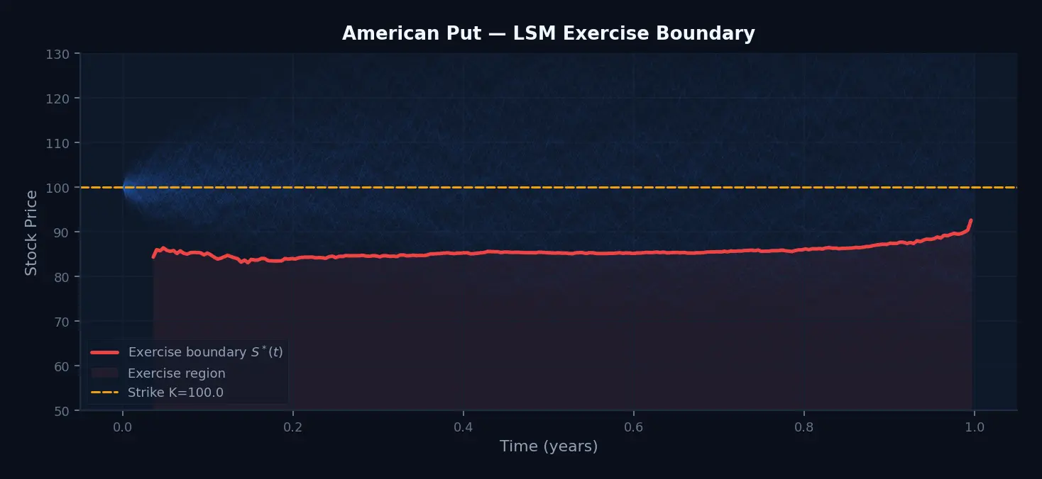
The backward induction not only gives us a price estimate; it also gives us an estimated exercise policy.

At each time step, there is a critical stock price $S^{*}$ below which an ITM put should be exercised immediately. Paths where $S_{t} < S^{*}$ should exercise; paths where $K > S_{t} > S^{*}$ should wait.

We can extract this boundary from the LSM runs:

def lsm_with_boundary(
    S0, K, r, sigma, T, n_steps, n_paths, degree=2, seed=42
):
    """LSM with exercise boundary tracking."""
    paths = simulate_paths(S0, r, sigma, T, n_steps, n_paths, seed)
    dt = T / n_steps
    discount = np.exp(-r * dt)
    payoff = np.maximum(K - paths, 0)
    cash_flow = payoff[:, -1].copy()

    boundary = np.full(n_steps + 1, np.nan)  # critical stock price per step

    for m in range(n_steps - 1, 0, -1):
        cash_flow *= discount
        S_m = paths[:, m]
        itm = payoff[:, m] > 0
        if itm.sum() < degree + 1:
            continue

        X = S_m[itm] / K
        Y = cash_flow[itm]
        basis = np.column_stack([X**k for k in range(degree + 1)])
        coeffs, _, _, _ = np.linalg.lstsq(basis, Y, rcond=None)
        continuation = basis @ coeffs

        exercise = payoff[itm, m] > continuation
        exercise_indices = np.where(itm)[0][exercise]

        if exercise_indices.size > 0:
            boundary[m] = paths[exercise_indices, m].max()

        cash_flow[exercise_indices] = payoff[exercise_indices, m]

    pv = discount * cash_flow
    intrinsic_now = max(K - S0, 0.0)
    if intrinsic_now > pv.mean():
        pv = np.full(n_paths, intrinsic_now)
    price = pv.mean()
    stderr = pv.std(ddof=1) / np.sqrt(n_paths)

    return price, stderr, boundary


price, se, boundary = lsm_with_boundary(S0, K, r, sigma, T, n_steps=252, n_paths=100_000)
times = np.linspace(0, T, 253)

# Inspect a few noisy, pathwise boundary estimates.
print(f"Price: {price:.4f} ± {1.96 * se:.4f}")
print(f"\nSample exercise boundary points:")
step_idx = [round(fraction * 252) for fraction in [0.1, 0.2, 0.4, 0.6, 0.8]]
for idx in step_idx:
    print(f"  t={times[idx]:.2f}y: largest exercised S ≈ {boundary[idx]:.2f}")

Price: 6.0555 ± 0.0437

Sample exercise boundary points:
  t=0.10y: largest exercised S ≈ 85.23
  t=0.20y: largest exercised S ≈ 83.99
  t=0.40y: largest exercised S ≈ 85.30
  t=0.60y: largest exercised S ≈ 85.12
  t=0.80y: largest exercised S ≈ 86.17

These are pathwise estimates, not an exact boundary. Taking the largest stock price exercised at each date produces sampling noise, so the raw sequence need not be monotone. The broader pattern is what matters: early in the option's life, the stock must be well below the strike before immediate exercise beats waiting; as expiry approaches and time value disappears, the theoretical boundary moves toward the strike.

The boundary is also model-dependent. Change volatility, rates, dividends, or the exercise-date grid and the estimated policy changes with it.

Estimated American put exercise boundary over time, shown as a red line above a shaded exercise region, with the strike marked at 100. — A smoothed LSM boundary estimate. Under this model, the exercise threshold trends upward as expiry approaches; raw pathwise estimates are noisier.

How Many Paths? The Convergence Picture

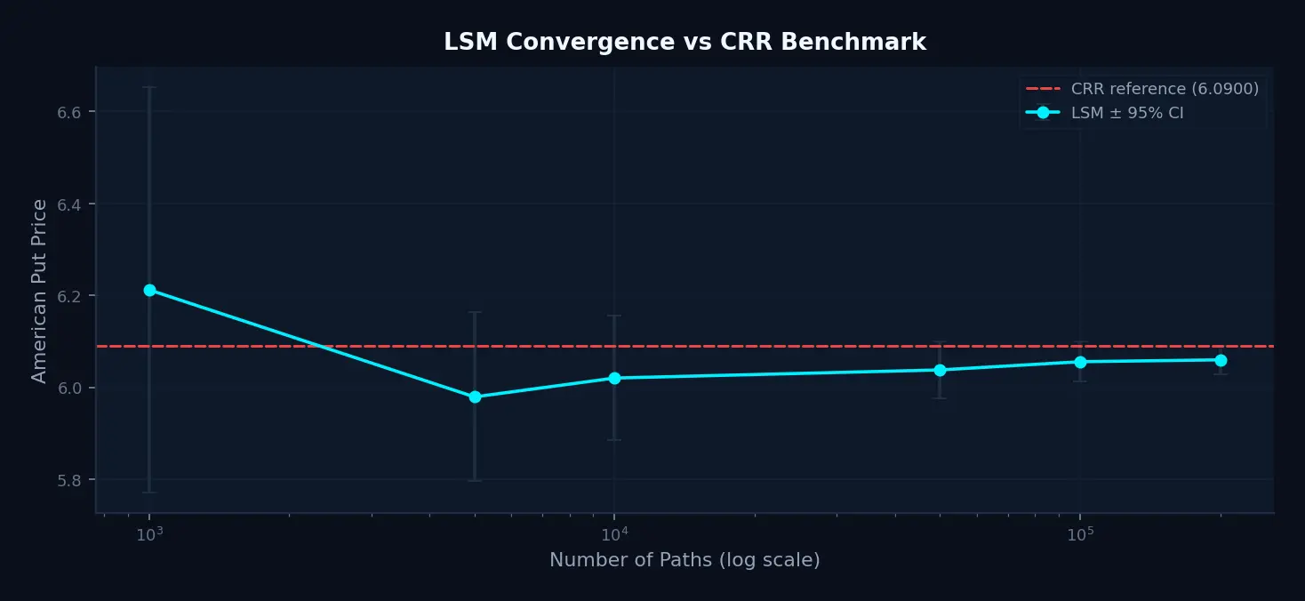
LSM has at least three numerical axes: more paths reduce sampling noise, more exercise dates reduce time-discretization error, and a better regression specification reduces continuation-value approximation error.

path_counts = [1_000, 5_000, 10_000, 50_000, 100_000, 200_000]
crr_ref = 6.0900  # crr_american_put(S0, K, r, sigma, T, n_steps=2000)

print(f"{'N paths':>12}  {'LSM price':>10}  {'±1.96 SE':>12}  {'vs CRR':>10}")
print("-" * 52)
for n in path_counts:
    p, se = lsm_american_put(S0, K, r, sigma, T, n_steps=252, n_paths=n, degree=2)
    print(f"{n:>12,}  {p:>10.4f}  ±{1.96*se:>9.4f}  {p - crr_ref:>+9.4f}")

print(f"\nCRR reference (2000 steps): {crr_ref:.4f}")

     N paths   LSM price      ±1.96 SE      vs CRR
----------------------------------------------------
       1,000      6.2118  ±   0.4414    +0.1218
       5,000      5.9789  ±   0.1838    -0.1111
      10,000      6.0200  ±   0.1358    -0.0700
      50,000      6.0376  ±   0.0616    -0.0524
     100,000      6.0555  ±   0.0437    -0.0345
     200,000      6.0596  ±   0.0310    -0.0304

CRR reference (2000 steps): 6.0900

The path-payoff sampling band shrinks at roughly the expected $1/ N$ rate. The point estimates are not monotone, and the remaining gap to CRR is larger than sampling noise alone at the highest path counts. That gap can reflect the finite exercise grid and the quadratic continuation-value approximation.

An estimated stopping rule cannot outperform the truly optimal rule when evaluated on independent paths, so policy approximation naturally produces a lower bound. This example reuses the same paths to fit and value the policy, however, so the printed standard error is descriptive rather than a complete error bound. A production study should fit the policy on one path set and evaluate it on another, or use a lower/upper-bound method.

For this one-factor benchmark, 50,000–100,000 paths and 50–252 exercise dates are enough to illustrate the method. That is not a universal production rule: path count, basis richness, exercise frequency, and validation design should be chosen for the contract and error tolerance.

Convergence chart showing the LSM price with plus-or-minus 1.96 path-payoff standard-error bars against the CRR benchmark as path count increases on a log scale. — LSM convergence against the CRR(2000) reference of 6.0900. The bars show path-payoff sampling error, not total pricing uncertainty.

The Basis Function Choice

The American-put example in the original paper uses a constant plus weighted Laguerre functions. The authors also report similar results with simple powers of the state variable. For a vanilla put, monomials such as $1$ , $S / K$ , and $(S / K)^{2}$ are an accessible starting point.

def lsm_with_laguerre(S0, K, r, sigma, T, n_steps, n_paths, seed=42):
    """LSM using a constant plus the first three weighted Laguerre functions."""
    paths = simulate_paths(S0, r, sigma, T, n_steps, n_paths, seed)
    dt = T / n_steps
    discount = np.exp(-r * dt)
    payoff = np.maximum(K - paths, 0)
    cash_flow = payoff[:, -1].copy()

    for m in range(n_steps - 1, 0, -1):
        cash_flow *= discount
        S_m = paths[:, m]
        itm = payoff[:, m] > 0
        if itm.sum() < 4:
            continue

        X = S_m[itm] / K  # the paper recommends normalization for stability
        Y = cash_flow[itm]

        weight = np.exp(-X / 2)
        basis = np.column_stack([
            np.ones_like(X),
            weight,
            weight * (1 - X),
            weight * (1 - 2*X + 0.5*X**2),
        ])
        coeffs, _, _, _ = np.linalg.lstsq(basis, Y, rcond=None)
        continuation = basis @ coeffs

        exercise = payoff[itm, m] > continuation
        exercise_indices = np.where(itm)[0][exercise]
        cash_flow[exercise_indices] = payoff[exercise_indices, m]

    pv = discount * cash_flow
    intrinsic_now = max(K - S0, 0.0)
    if intrinsic_now > pv.mean():
        pv = np.full(n_paths, intrinsic_now)
    return pv.mean(), pv.std(ddof=1) / np.sqrt(n_paths)


poly_price, poly_se = lsm_american_put(S0, K, r, sigma, T, n_steps=252, n_paths=100_000, degree=2)
lag_price,  lag_se  = lsm_with_laguerre(S0, K, r, sigma, T, n_steps=252, n_paths=100_000)

print(f"Polynomial basis:           {poly_price:.4f} ± {1.96*poly_se:.4f}")
print(f"Laguerre basis:             {lag_price:.4f}  ± {1.96*lag_se:.4f}")
print(f"CRR reference:              {crr_ref:.4f}")

Polynomial basis:           6.0555 ± 0.0437
Laguerre basis:             6.0848  ± 0.0440
CRR reference:              6.0900

Both specifications are close to the CRR benchmark, and the weighted Laguerre specification is closer in this particular run. That does not establish that it is universally superior. The two designs span different finite function spaces, and using the same simulated paths means their difference is not independent Monte Carlo noise; it is primarily a policy-specification difference on a shared sample.

A few practical notes on basis selection:

Include only ITM paths in the regression. Out-of-the-money paths add noise without helping — they would not exercise anyway.
Normalize the stock price (divide by $K$ or $S_{0}$ ) for better numerical conditioning.
Start with a small basis, then test richer alternatives against a trusted benchmark or on independently simulated valuation paths.
More functions can reduce approximation bias but increase estimation variance and numerical instability. There is no universally best count.

The Early Exercise Premium Across Parameters

The LSM algorithm lets us easily explore how the early exercise premium varies with the option's characteristics.

def early_exercise_premium(S0, K, r, sigma, T, n_steps=252, n_paths=100_000):
    euro = black_scholes_european_put(S0, K, r, sigma, T)
    amer, _ = lsm_american_put(S0, K, r, sigma, T, n_steps, n_paths, degree=2)
    return euro, amer, amer - euro


print(f"{'Scenario':<28} {'Euro Put':>9} {'Amer Put':>9} {'Premium':>9}")
print("-" * 60)

# Varying rate
for r_val in [0.01, 0.03, 0.05, 0.10]:
    euro, amer, prem = early_exercise_premium(100, 100, r_val, 0.20, 1.0)
    print(f"r={r_val:.2f}, σ=20%, ATM         {euro:>9.4f} {amer:>9.4f} {prem:>9.4f}")

print()
# Varying moneyness
for s in [120, 110, 100, 90, 80, 70]:
    euro, amer, prem = early_exercise_premium(s, 100, 0.05, 0.20, 1.0)
    label = "ITM" if s < 100 else ("ATM" if s == 100 else "OTM")
    print(f"S={s} ({label:3s}), r=5%, σ=20%    {euro:>9.4f} {amer:>9.4f} {prem:>9.4f}")

Scenario                     Euro Put  Amer Put   Premium
------------------------------------------------------------
r=0.01, σ=20%, ATM         7.4383    7.4915    0.0532
r=0.03, σ=20%, ATM         6.4580    6.7220    0.2640
r=0.05, σ=20%, ATM         5.5735    6.0555    0.4819
r=0.10, σ=20%, ATM         3.7534    4.7748    1.0213

S=120 (OTM), r=5%, σ=20%    1.2920    1.3597    0.0677
S=110 (OTM), r=5%, σ=20%    2.7859    2.9747    0.1888
S=100 (ATM), r=5%, σ=20%    5.5735    6.0555    0.4819
S=90  (ITM), r=5%, σ=20%   10.2142   11.4299    1.2157
S=80  (ITM), r=5%, σ=20%   16.9824   20.0000    3.0176
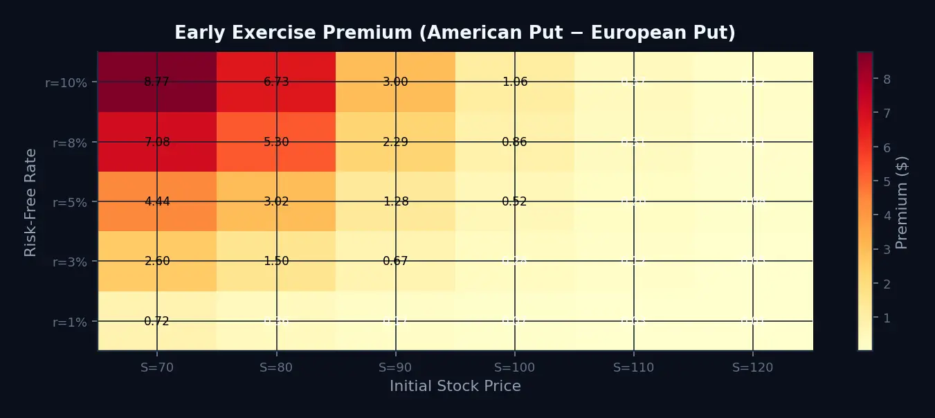
S=70  (ITM), r=5%, σ=20%   25.5644   30.0000    4.4356

Two clean patterns:

Higher rates → larger premium. For a put, early exercise realizes the strike component sooner; the financing benefit grows as rates rise. In this simulation, the estimated premium at $r = 10%$ is more than double the estimate at $r = 5%$ .

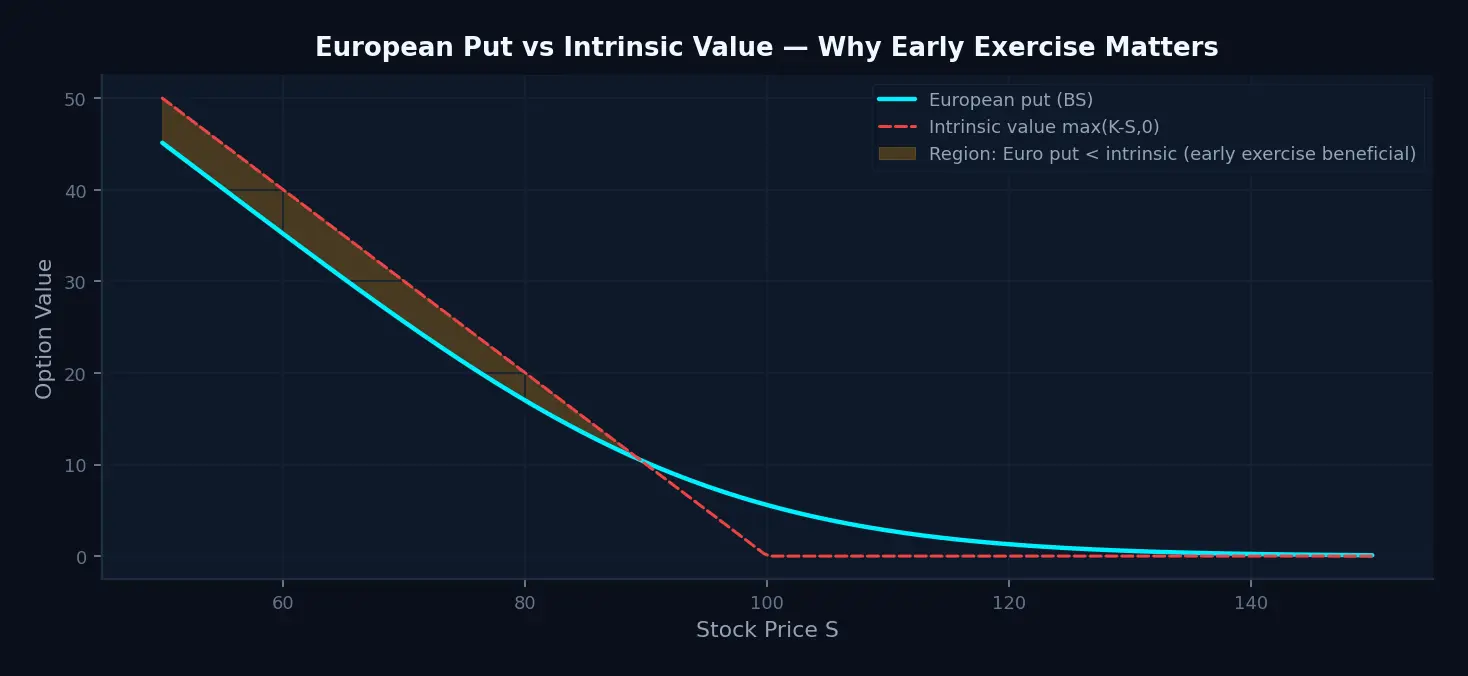
Deeper in the money → larger premium. When the stock is at 70 and the strike is 100, the intrinsic value is 30 and the European put is worth about 25.56. A European put can be worth less than current intrinsic value because it cannot be exercised before expiry and the strike is paid later. An American put is worth at least its immediate exercise value, so the code explicitly compares the rolled-back continuation estimate with intrinsic value at $t = 0$ . For $S_{0} = 80$ and $S_{0} = 70$ here, immediate exercise wins.

European put value and immediate exercise value across stock prices, with the region where intrinsic value is higher shaded. — A European put may lie below current intrinsic value because early exercise is unavailable. An American put cannot: immediate exercise supplies the floor.

Beyond Vanilla: Bermudan Options

The Longstaff-Schwartz algorithm extends naturally to Bermudan options — products with a fixed set of discrete exercise dates rather than continuous American exercise.

Bermudan-style exercise schedules appear in several markets:

Bermudan swaptions grant the right to enter a swap on any of a specified set of dates.
Callable bonds and cancelable swaps can contain issuer or counterparty options exercisable on contractual dates.
Convertible and employee-option contracts may combine exercise windows with vesting, call, or other path-dependent constraints. Those features require more state variables than the simple put below.

The core modification for a plain Bermudan put is small: make exercise decisions only on permitted dates. Real contracts can add notice periods, coupons, call rights, vesting, or path dependence, so their state representation is not trivial.

def lsm_bermudan_put(
    S0, K, r, sigma, T,
    exercise_dates: list[float],
    n_steps_per_year=52,
    n_paths=100_000,
    degree=2,
    seed=42,
):
    """
    Price a Bermudan put with exercise allowed only on specified dates.
    exercise_dates: times in [0, T] when exercise is permitted.
    """
    n_steps = int(T * n_steps_per_year)
    dt = T / n_steps
    paths = simulate_paths(S0, r, sigma, T, n_steps, n_paths, seed)
    payoff = np.maximum(K - paths, 0)
    cf_matrix = np.zeros_like(paths)
    cf_matrix[:, -1] = payoff[:, -1]

    if any(ed < 0 or ed > T for ed in exercise_dates):
        raise ValueError("exercise dates must lie in [0, T]")

    # Convert exercise dates to unique step indices.
    exercise_steps = sorted(
        {round(ed / dt) for ed in exercise_dates},
        reverse=True,
    )

    for m in exercise_steps:
        if m in (0, n_steps):
            continue   # handle expiry and t=0 outside the regression loop
        S_m = paths[:, m]
        itm = payoff[:, m] > 0
        if itm.sum() < degree + 1:
            continue

        future_cf = np.zeros(n_paths)
        for k in range(m + 1, n_steps + 1):
            future_cf += cf_matrix[:, k] * np.exp(-r * (k - m) * dt)

        X = S_m[itm] / K
        Y = future_cf[itm]
        basis = np.column_stack([X**k for k in range(degree + 1)])
        coeffs, _, _, _ = np.linalg.lstsq(basis, Y, rcond=None)
        continuation = basis @ coeffs

        exercise = payoff[itm, m] > continuation
        exercise_indices = np.where(itm)[0][exercise]
        cf_matrix[exercise_indices, m] = payoff[exercise_indices, m]
        cf_matrix[exercise_indices, m + 1:] = 0.0

    times = np.arange(n_steps + 1) * dt
    discount_factors = np.exp(-r * times)
    pv = (cf_matrix * discount_factors[np.newaxis, :]).sum(axis=1)
    if 0 in exercise_steps:
        intrinsic_now = max(K - S0, 0.0)
        if intrinsic_now > pv.mean():
            pv = np.full(n_paths, intrinsic_now)
    return pv.mean(), pv.std(ddof=1) / np.sqrt(n_paths)


# Quarterly exercise dates (0.25, 0.5, 0.75, 1.0)
quarterly_dates = [0.25, 0.5, 0.75, 1.0]
monthly_dates = [m / 12 for m in range(1, 13)]

berm_price, berm_se = lsm_bermudan_put(
    S0, K, r, sigma, T,
    exercise_dates=quarterly_dates,
    n_steps_per_year=52,
    n_paths=100_000,
)
monthly_price, monthly_se = lsm_bermudan_put(
    S0, K, r, sigma, T,
    exercise_dates=monthly_dates,
    n_steps_per_year=52,
    n_paths=100_000,
)

print(f"European put (no early exercise):  {euro_put:.4f}")
print(f"Bermudan put (quarterly):          {berm_price:.4f} ± {1.96*berm_se:.4f}")
print(f"Bermudan put (monthly):            {monthly_price:.4f} ± {1.96*monthly_se:.4f}")
print(f"American put (252-step approx):    {lsm_price:.4f} ± {1.96*lsm_se:.4f}")

European put (no early exercise):  5.5735
Bermudan put (quarterly):          5.9089 ± 0.0467
Bermudan put (monthly):            5.9837 ± 0.0451
American put (252-step approx):    6.0555 ± 0.0437

The Bermudan put sits between the European and the 252-step American approximation, as expected. Monthly exercise is more valuable than quarterly, and more exercise opportunities push it toward the 252-step American benchmark.

The framework extends to other payoffs and multiple risk factors, but the code does not do that automatically. A multi-factor implementation must simulate every relevant state variable and supply basis functions rich enough to approximate continuation value from that state.

Heatmap showing the early exercise premium for an American put across initial stock prices from 70 to 120 and risk-free rates from 1% to 10%. The premium is largest in the upper-left region, where rates are high and the put is deep in the money. — CRR benchmark for the early exercise premium across stock prices and risk-free rates. Deep in-the-money and high-rate cases produce the largest premium in this parameter grid.

Where LSM Fits

LSM is most attractive when simulation is already natural and a lattice or PDE becomes awkward because the contract is path-dependent or driven by several state variables. The original paper demonstrates that range rather than merely asserting it:

A cancelable index-amortizing swap with path-dependent cash flows.
An American put under jump diffusion, where the state distribution is no longer lognormal.
A deferred American swaption in a 20-factor term-structure model.

The same architecture can be adapted to callable structures, storage and swing options, mortgage-related optionality, and other real-option problems. Those are applications of the framework, not evidence that one quadratic regression is sufficient. Each requires contract-specific state variables, cash-flow logic, exercise constraints, and validation.

LSM is also not the automatic best choice for every American option. A one-factor vanilla put may be priced faster and more transparently with a tree or finite-difference solver. Simulation becomes compelling when its flexibility offsets the extra regression and validation risk.

The common thread is a choice between acting now and waiting, combined with a state process that can be simulated and represented well enough for regression.

CRR vs. FDM vs. LSM: A Practical Comparison

This series has now solved the same American put three ways: a lattice (Part 2), a PDE grid (Part 3), and simulation plus regression (this post). None dominates the other two — they trade accuracy, dimensionality, and error control differently.

	CRR / Leisen-Reimer tree	Crank-Nicolson + PSOR	Longstaff-Schwartz
Discretizes	the stock-price process (a lattice)	the Black-Scholes PDE (a grid)	nothing structural — simulates paths, then regresses continuation value
Rollback cost	$O (N)$ work at each of $N$ steps → $O (N^{2})$ total	$O (N_{S})$ per PSOR sweep (tridiagonal), tens to hundreds of sweeps per time step	$O (N_{p a t h s})$ per exercise date for path generation and OLS
Convergence character	odd/even sawtooth for plain CRR; substantially smoother with Leisen-Reimer or Tian	$O (Δ S^{2} + Δ τ^{2})$ where the solution is smooth, degraded by the payoff kink and domain truncation	$O (1/ N_{p a t h s})$ statistical error, plus basis-approximation and exercise-grid bias
Error is controlled by	one axis: step count	four separable axes: domain truncation, spatial grid, time grid, PSOR tolerance	three axes: path count, exercise-date density, basis richness
Risk factors	one, awkwardly two — state count then explodes	one, awkwardly two — same curse of dimensionality	scales polynomially in the number of factors, not exponentially — the reason the method exists
Path-dependent payoffs	break recombination	require augmenting the PDE state	natural — the realized cash flow is whatever the path produced
Exercise boundary	read directly off lattice nodes	read directly off grid nodes	reconstructed from the fitted regression; noisier, as shown above

A single-machine, illustrative timing check at the settings each post actually used — CRR at 1,000 steps, CN-PSOR at a 100×100 grid, LSM at 252 steps and 100,000 paths — put CRR around 0.01s, CN-PSOR around 0.06s, and LSM around 2.3s. Take that ordering, not the absolute numbers, as the takeaway: for a plain 1D put, the tree and the grid are both faster and land closer to the CRR(2000) reference than LSM does at these settings. The PSOR loop here is also unvectorized Python written for clarity, not a tuned production LCP solver — the FDM post already notes that direct or penalty-based solvers can be materially faster.

General guidelines:

Vanilla, single-factor American puts or calls, and you want a quick, transparent, cent-accurate price. Reach for the CRR or Leisen-Reimer tree. It has one convergence knob, backward induction is easy to reason about, and it is the natural teaching tool.
A single- or two-factor contract where you need separately controllable error bars, or where local-volatility or dividend-schedule flexibility matters. Reach for Crank-Nicolson with PSOR. The PDE/LCP framework lets you isolate domain, grid, time-step, and iteration error independently, and the free boundary falls out of the converged grid.
The contract is path-dependent (Asian, lookback, cliquet features), driven by more than two risk factors, or the underlying process is not a simple lognormal lattice — jump-diffusion, stochastic volatility, multi-factor term structure. Reach for Longstaff-Schwartz. This is precisely where recombining lattices and PDE grids stop being practical, and where LSM's polynomial scaling in the number of state variables pays for its extra simulation and regression cost.
You need a defensible, low-bias reference price for a high-stakes one- or two-factor contract. Prefer a fine tree or grid, or pair LSM with an independent out-of-sample valuation set (or a Broadie-Glasserman-style lower/upper bound pair). A single LSM run that fits and prices on the same paths is a biased, not a rigorous, estimate — a point this post has repeated for a reason.

The Takeaway

Continuously exercisable American options are hard because they embed a continuum of possible stopping times. A numerical implementation approximates that continuum with a finite exercise grid.

The Longstaff-Schwartz algorithm resolves this through one elegant observation:

The continuation value is a conditional expectation. A conditional expectation can be approximated by regression. And regression is computable from simulated data.

That chain of reasoning converts a backward-looking optimal stopping problem into a tractable forward simulation followed by a backward regression sweep.

The idea extends beyond vanilla puts, but flexibility is not automatic accuracy. You must be able to simulate the relevant state, express every cash flow and exercise constraint, choose an adequate regression basis, and validate the resulting stopping policy.

This completes the core option pricing arc of this series. We started with geometric Brownian motion — a model for how stock prices move. We used Itô's lemma to derive the Black-Scholes PDE. We showed how Monte Carlo prices European-style claims by averaging discounted simulated payoffs. And now we've shown how regression adds an estimated stopping policy for early-exercise claims.

The next thread turns from pricing individual instruments to measuring the risk of portfolios.

Value at Risk in Python: Rolling Volatility, EWMA, and Breach Testing is next.

Companion Notebook

The Python notebook for this post is available for download: american-options-longstaff-schwartz.ipynb. It includes:

Full LSM implementation, benchmarked against CRR and Black-Scholes
Exercise boundary extraction and visualisation
Path-count convergence study against the CRR reference
Polynomial vs. weighted-Laguerre basis comparison
Bermudan pricing and the early exercise premium heatmap across rates and moneyness
Exercises covering dividends, higher-degree bases, and a multi-asset Bermudan basket put

Previous Posts in This Thread

American Options Series:

The American Option Problem: Why Early Exercise Has No Closed Form — optimal stopping, the free boundary, and the LCP formulation.
Binomial Trees for American Puts: CRR, Convergence, and Leisen-Reimer — backward induction on a discrete lattice.
Finite Differences and PSOR: Solving the American Put PDE — Crank-Nicolson and Projected SOR.

Earlier in the Randomness to Risk series:

Monte Carlo Option Pricing: When Closed Forms Stop Helping introduces path-dependent options, variance reduction, and the core MC pricing loop.
Black-Scholes Without the Magic: Turning Random Paths into a Pricing Equation derives the PDE and explains where closed forms come from.
Geometric Brownian Motion in Python: The First Model Every Quant Learns builds GBM paths from scratch.
From Itô to Black-Scholes: How Randomness Became a Pricing Engine traces the road from stochastic calculus to the pricing formula.

References

Francis A. Longstaff and Eduardo S. Schwartz, "Valuing American Options by Simulation: A Simple Least-Squares Approach", Review of Financial Studies, 14(1), 2001.
James A. Tilley, "Valuing American Options in a Path Simulation Model", Transactions of the Society of Actuaries, 45, 1993.
Jacques F. Carriere, "Valuation of the Early-Exercise Price for Options Using Simulations and Nonparametric Regression", Insurance: Mathematics and Economics, 19(1), 1996.
Mark Broadie and Paul Glasserman, "Pricing American-Style Securities Using Simulation", Journal of Economic Dynamics and Control, 21, 1997.
John C. Cox, Stephen A. Ross, and Mark Rubinstein, "Option Pricing: A Simplified Approach", Journal of Financial Economics, 7(3), 1979.
Fischer Black and Myron Scholes, "The Pricing of Options and Corporate Liabilities", Journal of Political Economy, 1973.
Robert C. Merton, "Theory of Rational Option Pricing", The Bell Journal of Economics and Management Science, 1973.

Get in Touch

Working on option pricing, structured products, or risk model development? Thinking through the CQF or building a quant research stack?

Connect with me:

📧 Email: [email protected]
🐦 Twitter/X: @TheDataGuyPro
💼 LinkedIn: Muhammad Afzaal
💻 GitHub: @mafzaal
🎥 YouTube: @TheDataGuyPro
🎧 Podcast: TheDataGuy Show

Whether you're studying for the CQF, building production pricing infrastructure, or exploring quant finance fundamentals, I'd love to hear from you!

Contents