Monte Carlo Option Pricing: When Closed Forms Stop Helping

The previous post ended with a cliff-hanger buried in a paragraph about limitations.

Black-Scholes gives us a clean formula for a European call or put. We worked hard for that formula — Itô's lemma, delta hedging, a PDE, a boundary condition. The payoff was a closed-form expression you could evaluate in a spreadsheet.

But then the post asked:

What happens when the payoff is too complicated for a clean formula?

That question is not hypothetical.

Real option markets are full of contracts where the payoff depends not just on where the stock finishes, but on everything it did along the way. Contracts that knock out if the stock touches a barrier. Contracts that pay based on the average stock price over six months. Contracts that lock in the best price seen over the life of the trade.

For all of these, the beautiful machinery that produced the Black-Scholes formula simply does not produce a usable answer.

The closed form stops helping.

And when that happens, you reach for Monte Carlo.

Monte Carlo option pricing is not a workaround. It is what happens when you take the risk-neutral pricing formula seriously and simulate it directly.

This is the fourth post in the Randomness to Risk series. It builds on geometric Brownian motion, Itô's lemma, and the risk-neutral pricing intuition from the earlier posts. If you haven't read those yet, the links are at the bottom of this page.

This is educational research. Nothing here is investment advice.

Want to run the examples locally? Download the companion Jupyter notebook.

The One Sentence That Contains the Whole Idea

Before diving into exotics and code, let's restate the risk-neutral pricing result from the last post.

Under the risk-neutral measure $Q$ , an option is worth its discounted expected payoff. For a European option — where the payoff depends only on the terminal stock price:

V (S_{t}, t) = e^{- r (T - t)} E^{Q} [Payoff (S_{T}) ∣ S_{t}]

For path-dependent options, the payoff is a functional of the entire path $Φ ((S_{u})_{u \in [t, T]})$ , and the formula generalises to conditioning on the full information set:

V_{t} = e^{- r (T - t)} E^{Q} [Φ ((S_{u})_{u \in [t, T]}) ∣ F_{t}]

For a European call, $Φ = max (S_{T} - K, 0)$ . The expectation over a log-normal distribution has a known closed form — that is Black-Scholes.

But this pricing principle does not care whether the payoff is simple.

It says: whatever the payoff looks like, the option price is its discounted expected value under the risk-neutral measure.

That expectation is an integral. For complicated payoffs, that integral has no closed form.

But an integral over many possible futures is exactly what a simulation can approximate.

The Monte Carlo idea fits naturally into this one sentence:

Simulate many stock paths under the risk-neutral measure.
Compute the payoff on each path.
Average the payoffs.
Discount the average.

That is it.

The result is a sample estimate of the integral we cannot evaluate analytically.

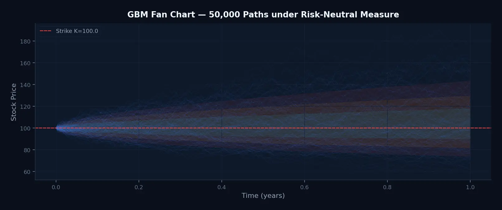
Simulating Risk-Neutral Paths

The risk-neutral stock price model from the previous posts is geometric Brownian motion with the expected return replaced by the risk-free rate $r$ :

d S_{t} = r S_{t} d t + σ S_{t} d W_{t}^{Q}

We discretize this exactly using the log-return formula we derived from Itô's lemma:

S_{t + Δ t} = S_{t} exp [(r - \frac{1}{2} σ^{2}) Δ t + σ Δ t Z]

where $Z \sim N (0, 1)$ .

Here is a clean Python implementation that generates a matrix of paths:

import numpy as np


def simulate_paths(
    S0: float,
    r: float,
    sigma: float,
    T: float,
    n_steps: int,
    n_paths: int,
    seed: int = 42,
) -> np.ndarray:
    """
    Simulate GBM paths under the risk-neutral measure.
    Returns array of shape (n_paths, n_steps + 1).
    """
    rng = np.random.default_rng(seed)
    dt = T / n_steps

    Z = rng.standard_normal((n_paths, n_steps))
    log_increments = (r - 0.5 * sigma**2) * dt + sigma * np.sqrt(dt) * Z

    log_paths = np.cumsum(log_increments, axis=1)
    log_paths = np.hstack([np.zeros((n_paths, 1)), log_paths])

    return S0 * np.exp(log_paths)

Notice the risk-neutral drift: we use r not mu. Under real-world measure we would use the stock's actual expected return. Under risk-neutral measure we use the risk-free rate. The reason is the same as before — we are pricing, not forecasting.

Let us also establish a basic Monte Carlo pricer template. Every option we price will follow this structure:

import numpy as np
from scipy.stats import norm


def mc_price(
    payoff_fn,
    S0: float,
    r: float,
    sigma: float,
    T: float,
    n_steps: int,
    n_paths: int,
    seed: int = 42,
) -> tuple[float, float]:
    """
    Generic Monte Carlo pricer.
    Returns (price estimate, standard error).
    """
    paths = simulate_paths(S0, r, sigma, T, n_steps, n_paths, seed)
    payoffs = payoff_fn(paths)
    discounted = np.exp(-r * T) * payoffs
    price = discounted.mean()
    stderr = discounted.std() / np.sqrt(n_paths)
    return price, stderr

We return both the price and its standard error. The standard error tells us how confident we should be in the estimate. This matters — a Monte Carlo price without a confidence interval is an incomplete answer.

GBM fan chart showing 200 simulated stock price paths under the risk-neutral measure, with percentile bands at the 10th, 25th, and 50th percentiles and the strike price marked. — 50,000 GBM paths under the risk-neutral measure. The strike K=100 is shown as a dashed line. Percentile bands show the distribution fanning out over one year.

The Baseline: Repricing a European Call

Before tackling exotics, let us verify the engine works by pricing something we can check analytically.

A European call has the payoff:

Payoff = max (S_{T} - K, 0)

This only depends on the final stock price $S_{T}$ , not the path.

def black_scholes_call(S0, K, r, sigma, T):
    d1 = (np.log(S0 / K) + (r + 0.5 * sigma**2) * T) / (sigma * np.sqrt(T))
    d2 = d1 - sigma * np.sqrt(T)
    return S0 * norm.cdf(d1) - K * np.exp(-r * T) * norm.cdf(d2)


def european_call_payoff(paths, K):
    return np.maximum(paths[:, -1] - K, 0)


# Parameters
S0, K, r, sigma, T = 100, 100, 0.05, 0.20, 1.0
n_steps, n_paths = 252, 100_000

bs_price = black_scholes_call(S0, K, r, sigma, T)

mc_est, mc_se = mc_price(
    payoff_fn=lambda p: european_call_payoff(p, K),
    S0=S0, r=r, sigma=sigma, T=T,
    n_steps=n_steps, n_paths=n_paths,
)

print(f"Black-Scholes: {bs_price:.4f}")
print(f"Monte Carlo:   {mc_est:.4f} ± {1.96 * mc_se:.4f}")

Black-Scholes: 10.4506
Monte Carlo:   10.4526 ± 0.1294

The Monte Carlo estimate falls within the 95% confidence interval of the analytic answer. The engine is honest.

This is an important exercise. When you use Monte Carlo for an exotic option where you cannot verify analytically, the confidence you have in the simulation comes from knowing it reprices the simple cases correctly.

The Trouble with Path

Now let us introduce the problem that makes Monte Carlo necessary.

Consider two stock paths starting at 100 and ending at 120 after one year.

Path A: the stock climbs steadily from 100 to 120.

Path B: the stock spikes to 150 in month three, falls to 80 in month eight, and recovers to 120 at expiry.

For a European call with strike 100, both paths produce the same payoff: 20. The path shape is irrelevant — only the terminal value matters.

But now imagine a different contract:

The option pays the average stock price over the year minus the strike.

Or:

The option is cancelled if the stock ever crosses 130.

Or:

The option pays the highest price observed over the year minus the strike.

Suddenly, Path A and Path B produce completely different payoffs. The path is the product.

This is the class of instruments known as path-dependent options, and it is where Black-Scholes in closed form can no longer follow.

Asian Options: The Path Average Matters

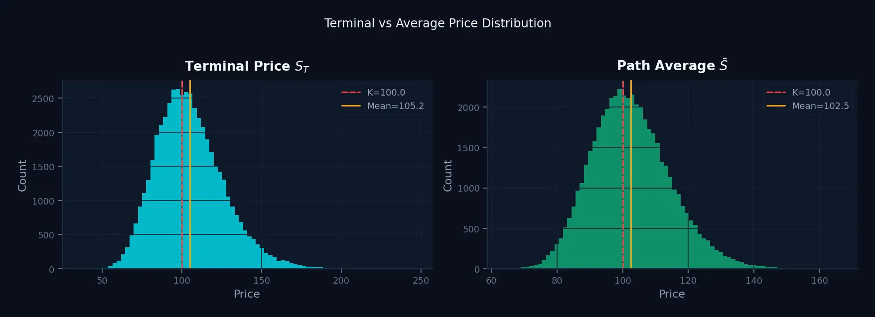
An Asian option is one of the most common exotics. Instead of the terminal price, the payoff uses the arithmetic average of the stock price over the life of the contract:

Payoff = max (S ˉ - K, 0) where S ˉ = \frac{1}{n} i = 1 \sum n S_{t_{i}}

Why does this exist?

Because many real markets — commodity contracts, currency-linked payments, employee stock option plans — settle against a price average rather than a single snapshot. A single day's closing price is easy to manipulate or distorted by temporary events. The average is harder to game.

Asian options are also cheaper than European options, because averaging reduces the effective volatility. A series of daily prices averages out some of the noise. That makes the distribution of the payoff tighter, and a tighter distribution of a capped payoff is worth less.

Pricing an Asian option with Monte Carlo is almost trivially different from pricing a European option. We just change what we do with the paths:

def asian_call_payoff(paths, K):
    # Average over all time steps (columns), not just the final
    avg_prices = paths[:, 1:].mean(axis=1)  # exclude t=0
    return np.maximum(avg_prices - K, 0)


asian_price, asian_se = mc_price(
    payoff_fn=lambda p: asian_call_payoff(p, K),
    S0=S0, r=r, sigma=sigma, T=T,
    n_steps=n_steps, n_paths=n_paths,
)

print(f"Asian call MC:  {asian_price:.4f} ± {1.96 * asian_se:.4f}")
print(f"European call:  {bs_price:.4f}")

Asian call MC:  5.7740 ± 0.0701
European call:  10.4506

The Asian call is roughly 45% cheaper. That is the averaging discount in action.

One line changed — paths[:, -1] became paths[:, 1:].mean(axis=1) — and we priced a product that has no elementary closed form. That is the power of this approach.

Side-by-side histograms comparing the distribution of terminal prices S_T versus path average prices S_bar, showing that the average is narrower and tighter around the mean. — Terminal price distribution vs path average distribution. The average is tighter — lower variance means a lower option price.

Barrier Options: Alive Until It Isn't

A barrier option has a clause that activates or deactivates the contract if the stock price crosses a threshold during the life of the trade.

The two most common varieties:

Knock-out: starts as a live option; dies if the stock touches the barrier. The holder receives a small rebate, or nothing.
Knock-in: starts dormant; only becomes live if the stock touches the barrier.

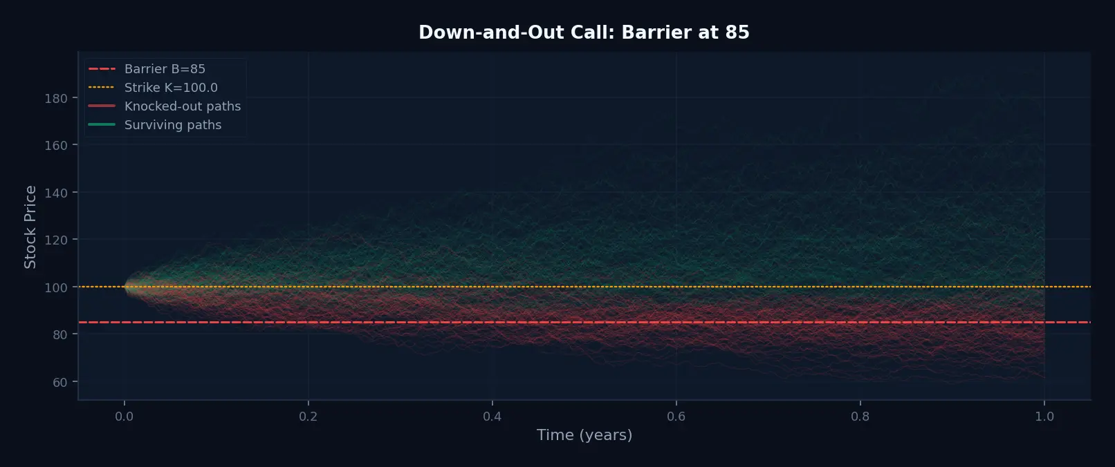
A down-and-out call starts like a regular call but disappears if the stock ever falls below the barrier $B$ :

Payoff = max (S_{T} - K, 0) \cdot 1 [0 \leq t \leq T min S_{t} > B]

Barrier options are widely used in structured products. They are cheaper than plain options because the holder accepts the risk of losing the option at the worst moment — when the stock is already falling.

Some barrier contracts have analytic formulas in the Black-Scholes world (Rubinstein and Reiner derived them in 1991). But those formulas assume continuous monitoring. In practice, barriers are monitored daily. And once you add stochastic volatility, jumps, or more complex barrier structures, the closed form breaks down.

Monte Carlo handles all of this naturally:

def down_and_out_call_payoff(paths, K, B):
    """Down-and-out call: knocked out if stock ever hits or drops below B."""
    alive = paths.min(axis=1) > B          # True if barrier never touched
    terminal_payoff = np.maximum(paths[:, -1] - K, 0)
    return terminal_payoff * alive


def down_and_in_call_payoff(paths, K, B):
    """Down-and-in call: only pays if stock touched the barrier."""
    touched = paths.min(axis=1) <= B
    terminal_payoff = np.maximum(paths[:, -1] - K, 0)
    return terminal_payoff * touched


B = 85  # barrier at 85

dao_price, dao_se = mc_price(
    payoff_fn=lambda p: down_and_out_call_payoff(p, K, B),
    S0=S0, r=r, sigma=sigma, T=T,
    n_steps=n_steps, n_paths=n_paths,
)
dai_price, dai_se = mc_price(
    payoff_fn=lambda p: down_and_in_call_payoff(p, K, B),
    S0=S0, r=r, sigma=sigma, T=T,
    n_steps=n_steps, n_paths=n_paths,
)

print(f"Down-and-out call: {dao_price:.4f} ± {1.96 * dao_se:.4f}")
print(f"Down-and-in call:  {dai_price:.4f} ± {1.96 * dai_se:.4f}")
print(f"Sum (should ≈ European): {dao_price + dai_price:.4f}")

Down-and-out call: 10.0489 ± 0.1299
Down-and-in call:   0.4037 ± 0.0224
Sum (should ≈ European): 10.4526

The sum check is a beautiful consistency test. A down-and-out plus a down-and-in with the same barrier and strike form a replication of a plain European call — because every path either hits the barrier or it doesn't. If the sum does not approximately equal the European price, something is wrong with the simulation.

Here, the sum is 10.4526 against the Black-Scholes price of 10.4506.

The barrier parity check is a free sanity test. If your knock-out plus knock-in does not equal the vanilla price, your simulation has a bug.

Fan chart of 300 sample paths, with knocked-out paths shown in red and surviving paths in green. The barrier at 85 and strike at 100 are marked. — Down-and-out call: paths that touch the barrier at 85 are knocked out (red). Surviving paths (green) collect the call payoff at expiry.

Lookback Options: The Best Price You Never Had

A lookback option is almost unfairly useful to the holder.

A floating-strike lookback call pays the difference between the terminal stock price and the minimum price seen over the contract's life:

Payoff = S_{T} - 0 \leq t \leq T min S_{t}

It is as if the holder had perfect hindsight about when to buy — they notionally bought at the lowest point.

A fixed-strike lookback call pays the maximum price over the life minus the strike:

Payoff = max (0 \leq t \leq T max S_{t} - K, 0)

Lookbacks are expensive because they guarantee the best outcome the path could have offered. They exist in practice primarily in exotic structured products. Their main value in this context is as a clean illustration that MC handles any path statistic with equal ease:

def lookback_floating_call_payoff(paths):
    """Pays terminal price minus observed minimum (monitoring all dates including t=0)."""
    return paths[:, -1] - paths.min(axis=1)


def lookback_fixed_call_payoff(paths, K):
    """Pays observed maximum minus strike (monitoring all dates including t=0)."""
    return np.maximum(paths.max(axis=1) - K, 0)


lb_float_price, lb_float_se = mc_price(
    payoff_fn=lookback_floating_call_payoff,
    S0=S0, r=r, sigma=sigma, T=T,
    n_steps=n_steps, n_paths=n_paths,
)
lb_fixed_price, lb_fixed_se = mc_price(
    payoff_fn=lambda p: lookback_fixed_call_payoff(p, K),
    S0=S0, r=r, sigma=sigma, T=T,
    n_steps=n_steps, n_paths=n_paths,
)

print(f"Lookback floating call: {lb_float_price:.4f} ± {1.96 * lb_float_se:.4f}")
print(f"Lookback fixed call:    {lb_fixed_price:.4f} ± {1.96 * lb_fixed_se:.4f}")
print(f"European call (ref):    {bs_price:.4f}")

Lookback floating call: 16.5925 ± 0.1277
Lookback fixed call:    18.3460 ± 0.1347
European call (ref):    10.4506

Both lookbacks are substantially more expensive than a standard European call. That is correct. The holder captures the best possible path outcome. The market prices that guarantee accordingly.

Three different exotic payoffs, all priced with the same simulation engine. The only thing that changed was one function.

The Convergence Problem

So far, Monte Carlo looks almost too easy.

It is not.

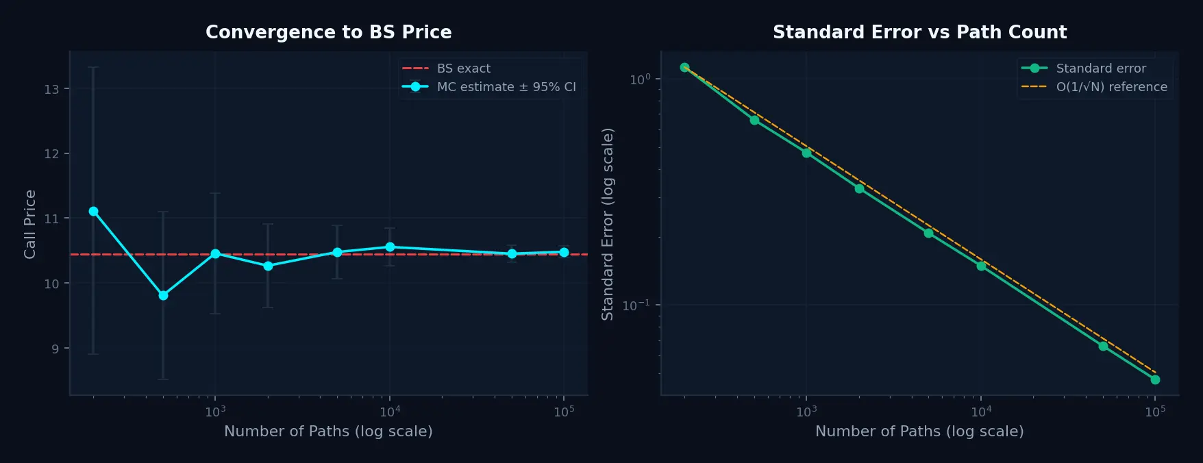
The price of Monte Carlo's generality is slow convergence.

For $N$ independent paths, the standard error of the Monte Carlo estimate scales as:

SE = \frac{σ _{payoff}}{N}

This is the $O (1/ N)$ convergence rate. To halve the error, you quadruple the number of paths.

Let us make this concrete:

def convergence_study(payoff_fn, S0, r, sigma, T, n_steps, max_paths=500_000):
    path_counts = [500, 1_000, 5_000, 10_000, 50_000, 100_000, 500_000]
    results = []

    for n in path_counts:
        price, se = mc_price(payoff_fn, S0, r, sigma, T, n_steps, n_paths=n)
        results.append({
            "n_paths": n,
            "price": price,
            "se": se,
            "ci_half_width": 1.96 * se,
        })

    return results


study = convergence_study(
    payoff_fn=lambda p: european_call_payoff(p, K),
    S0=S0, r=r, sigma=sigma, T=T, n_steps=252,
)

for row in study:
    print(
        f"N={row['n_paths']:>7,}  "
        f"price={row['price']:.4f}  "
        f"95% CI width ±{row['ci_half_width']:.4f}"
    )

N=    500  price=9.8101  95% CI width ±1.2934
N=  1,000  price=10.4585  95% CI width ±0.9266
N=  5,000  price=10.4789  95% CI width ±0.4088
N= 10,000  price=10.5575  95% CI width ±0.2928
N= 50,000  price=10.4526  95% CI width ±0.1294
N=100,000  price=10.4829  95% CI width ±0.0919
N=500,000  price=10.4832  95% CI width ±0.0409

Notice the pattern. Going from 1,000 to 100,000 paths — a factor of 100 more work — improves precision by a factor of 10. The square root appears in the denominator. You pay dearly for every extra decimal place.

For a simple European call, this is wasteful. Black-Scholes gives us the answer in microseconds.

For a path-dependent exotic, there is no choice.

Two-panel chart: left shows MC price convergence to the Black-Scholes value as N increases; right shows standard error decreasing on a log-log scale with an O(1/sqrt(N)) reference line. — Left: MC estimate converges to the Black-Scholes price as paths increase. Right: standard error tracks the O(1/√N) slope on a log-log axis.

Variance Reduction: Getting More Accuracy Per Path

Because raw Monte Carlo converges slowly, practitioners deploy variance reduction techniques — methods that reduce $σ_{payoff}$ without biasing the estimate.

The two most accessible methods are antithetic variates and control variates.

Antithetic Variates: The Mirror Trick

For every random draw $Z$ , we also evaluate the payoff using $- Z$ .

If $Z$ causes a high path, $- Z$ causes a low path. The two payoffs tend to be negatively correlated. Their average has lower variance than either alone.

def mc_price_antithetic(
    payoff_fn,
    S0: float,
    r: float,
    sigma: float,
    T: float,
    n_steps: int,
    n_paths: int,
    seed: int = 42,
) -> tuple[float, float]:
    """Monte Carlo with antithetic variates."""
    rng = np.random.default_rng(seed)
    dt = T / n_steps
    n_half = n_paths // 2

    Z = rng.standard_normal((n_half, n_steps))
    log_inc = (r - 0.5 * sigma**2) * dt + sigma * np.sqrt(dt) * Z
    log_inc_anti = (r - 0.5 * sigma**2) * dt + sigma * np.sqrt(dt) * (-Z)

    def build_paths(increments):
        lp = np.hstack([np.zeros((n_half, 1)), np.cumsum(increments, axis=1)])
        return S0 * np.exp(lp)

    payoffs_orig = payoff_fn(build_paths(log_inc))
    payoffs_anti = payoff_fn(build_paths(log_inc_anti))

    # Average each antithetic pair before computing the overall mean
    paired_payoffs = 0.5 * (payoffs_orig + payoffs_anti)
    discounted = np.exp(-r * T) * paired_payoffs
    price = discounted.mean()
    stderr = discounted.std() / np.sqrt(n_half)
    return price, stderr


plain_price, plain_se = mc_price(
    lambda p: european_call_payoff(p, K),
    S0, r, sigma, T, n_steps=252, n_paths=10_000,
)
anti_price, anti_se = mc_price_antithetic(
    lambda p: european_call_payoff(p, K),
    S0, r, sigma, T, n_steps=252, n_paths=10_000,
)

print(f"Plain MC:       price={plain_price:.4f}, SE={plain_se:.4f}")
print(f"Antithetic MC:  price={anti_price:.4f}, SE={anti_se:.4f}")
print(f"SE reduction:   {plain_se / anti_se:.2f}x improvement")

Plain MC:       price=10.5575, SE=0.1494
Antithetic MC:  price=10.2988, SE=0.1010
SE reduction:   1.48x improvement

For the same 10,000 paths, antithetic variates reduced the standard error by about 32% — equivalent to roughly 2.2× more paths for free.

Control Variates: Using What You Know

When you have a related quantity with a known analytic value, you can use the relationship between the simulation estimate and the known value to correct your estimate.

Suppose we are pricing an Asian call but we can also compute the European call price analytically. The Asian and European calls on the same stock are correlated — paths that produce high European payoffs tend to produce high Asian payoffs too.

The control variate correction works as follows:

Compute both the Asian payoff and the European payoff on each simulated path.
Note that the simulated European payoff has a known expectation: the Black-Scholes price.
If the simulation overestimates the European price, it likely overestimates the Asian price by a similar amount. Subtract the error.

def mc_price_control_variate(
    S0: float,
    r: float,
    sigma: float,
    T: float,
    K: float,
    n_steps: int,
    n_paths: int,
    seed: int = 42,
) -> tuple[float, float]:
    """Price Asian call using European call as control variate."""
    paths = simulate_paths(S0, r, sigma, T, n_steps, n_paths, seed)
    discount = np.exp(-r * T)

    asian_payoffs = discount * np.maximum(paths[:, 1:].mean(axis=1) - K, 0)
    euro_payoffs  = discount * np.maximum(paths[:, -1] - K, 0)

    bs_exact = black_scholes_call(S0, K, r, sigma, T)

    # Optimal coefficient (regression of target on control)
    cov = np.cov(asian_payoffs, euro_payoffs)
    beta = cov[0, 1] / cov[1, 1]

    # Adjusted estimate
    adjusted = asian_payoffs - beta * (euro_payoffs - bs_exact)
    price = adjusted.mean()
    stderr = adjusted.std() / np.sqrt(n_paths)
    return price, stderr


plain_asian, plain_asian_se = mc_price(
    lambda p: asian_call_payoff(p, K),
    S0, r, sigma, T, n_steps=252, n_paths=10_000,
)
cv_asian, cv_asian_se = mc_price_control_variate(
    S0, r, sigma, T, K, n_steps=252, n_paths=10_000,
)

print(f"Asian plain MC:     price={plain_asian:.4f}, SE={plain_asian_se:.4f}")
print(f"Asian + CV:         price={cv_asian:.4f}, SE={cv_asian_se:.4f}")
print(f"SE reduction:       {plain_asian_se / cv_asian_se:.2f}x improvement")

Asian plain MC:     price=5.7740, SE=0.0358
Asian + CV:         price=5.7731, SE=0.0193
SE reduction:       1.85x improvement

The control variate cut the standard error by more than half again. That 1.85x improvement comes from exploiting a known relationship rather than simulating blind.

Quasi-Monte Carlo: Replace Randomness with Covering

Standard Monte Carlo uses pseudo-random draws. These are good at avoiding patterns — but they can cluster accidentally, leaving gaps in the sample space.

Quasi-Monte Carlo (QMC) replaces random draws with low-discrepancy sequences — deterministic sequences designed to cover the sample space more uniformly. The most popular is the Sobol sequence.

Under QMC, convergence improves from $O (1/ N)$ toward $O ((lo g N)^{d} / N)$ for $d$ dimensions, which for moderate dimensions and large $N$ is meaningfully faster.

from scipy.stats import qmc

def simulate_paths_sobol(
    S0: float,
    r: float,
    sigma: float,
    T: float,
    n_steps: int,
    n_paths: int,
    seed: int = 42,
) -> np.ndarray:
    """GBM paths using Sobol quasi-random numbers (via normal transform)."""
    sampler = qmc.Sobol(d=n_steps, scramble=True, seed=seed)
    uniform = sampler.random(n_paths)          # (n_paths, n_steps) in [0,1)
    Z = norm.ppf(np.clip(uniform, 1e-10, 1 - 1e-10))  # normal quantiles

    dt = T / n_steps
    log_inc = (r - 0.5 * sigma**2) * dt + sigma * np.sqrt(dt) * Z
    log_paths = np.hstack([np.zeros((n_paths, 1)), np.cumsum(log_inc, axis=1)])
    return S0 * np.exp(log_paths)


n_paths_qmc = 4096  # Sobol works best with powers of 2

paths_sobol = simulate_paths_sobol(S0, r, sigma, T, n_steps=252, n_paths=n_paths_qmc)
euro_payoffs_qmc = np.exp(-r * T) * np.maximum(paths_sobol[:, -1] - K, 0)
qmc_price = euro_payoffs_qmc.mean()
qmc_se    = euro_payoffs_qmc.std() / np.sqrt(n_paths_qmc)

# Compare with plain MC at same path count
plain_price_4k, plain_se_4k = mc_price(
    lambda p: european_call_payoff(p, K),
    S0, r, sigma, T, n_steps=252, n_paths=n_paths_qmc,
)

print(f"Plain MC (N=4096):  price={plain_price_4k:.4f}, SE={plain_se_4k:.4f}")
print(f"QMC Sobol (N=4096): price={qmc_price:.4f},  sample dispersion={qmc_se:.4f}")
print(f"Black-Scholes:      price={bs_price:.4f}")

Plain MC (N=4096):  price=10.3687, SE=0.2313
QMC Sobol (N=4096): price=10.4163,  sample dispersion=0.2275
Black-Scholes:      price=10.4506

At 4,096 paths, QMC produces a tighter estimate than plain Monte Carlo. The Sobol sequence's uniform coverage gives us more signal per path. Note: for a single scrambled Sobol run, $σ^_{payoff} / N$ approximates integration error but is not a classical standard error — use multiple independent scramblings to estimate true dispersion.

When Not to Use Monte Carlo

Monte Carlo is powerful. It is also expensive, and it carries statistical noise that analytic methods do not have.

Knowing when not to use it is as important as knowing how to use it.

Use Black-Scholes (and its extensions) directly when:

The option has a known closed-form solution.
You need Greeks to machine precision — Black-Scholes Greeks are analytic; Monte Carlo Greeks require bump-and-reprice or pathwise sensitivity, both of which amplify variance.
You are doing real-time pricing under market stress. At a delta-hedging desk, computing 100,000 paths per price quote is not viable.
You are calibrating a model to market data — the optimiser calls the pricer thousands of times, and a noisy Monte Carlo estimate causes calibration instability.

Use Monte Carlo when:

The payoff depends on the path (Asian, barrier, lookback, cliquet, variance swaps).
The underlying follows a more realistic model — stochastic volatility (Heston), jump diffusion (Merton), stochastic interest rates — that has no tractable closed form.
You are computing credit valuation adjustment (CVA) or exposure profiles, which require joint simulation of market factors and counterparty defaults over time.
The product has multiple underlyings with correlated paths (basket options, worst-of structures, correlation swaps).

The clean rule:

If the payoff only depends on the terminal value and the model is log-normal, Black-Scholes is faster, cleaner, and exact. Monte Carlo enters the moment the path or the model becomes too complex for a formula.

Confidence Intervals in Practice

Every Monte Carlo result is an estimate, not a fact. The 95% confidence interval:

V^\pm 1.96 \cdot \frac{σ ^ _{payoff}}{N}

tells you the range that would capture the true price 95% of the time if you repeated the simulation with different random seeds.

A practical reporting discipline: always report the confidence interval alongside the price. A Monte Carlo price without error bars is like measuring the temperature to the nearest degree and reporting it to three decimal places.

Here is a function that does this properly, with a summary table:

def price_all_options(S0, K, B, r, sigma, T, n_steps, n_paths):
    bs = black_scholes_call(S0, K, r, sigma, T)

    results = {
        "European Call (BS)":        (bs, 0.0),
        "European Call (MC)":        mc_price(lambda p: european_call_payoff(p, K), S0, r, sigma, T, n_steps, n_paths),
        "Asian Call":                mc_price(lambda p: asian_call_payoff(p, K), S0, r, sigma, T, n_steps, n_paths),
        "Down-and-Out Call (B=85)":  mc_price(lambda p: down_and_out_call_payoff(p, K, B), S0, r, sigma, T, n_steps, n_paths),
        "Down-and-In Call (B=85)":   mc_price(lambda p: down_and_in_call_payoff(p, K, B), S0, r, sigma, T, n_steps, n_paths),
        "Lookback Float Call":       mc_price(lookback_floating_call_payoff, S0, r, sigma, T, n_steps, n_paths),
        "Lookback Fixed Call":       mc_price(lambda p: lookback_fixed_call_payoff(p, K), S0, r, sigma, T, n_steps, n_paths),
    }

    print(f"{'Option':<30} {'Price':>8}  {'95% CI':>14}")
    print("-" * 58)
    for name, (price, se) in results.items():
        ci = f"±{1.96 * se:.4f}" if se > 0 else "  (exact)"
        print(f"{name:<30} {price:>8.4f}  {ci:>14}")


price_all_options(S0=100, K=100, B=85, r=0.05, sigma=0.20, T=1.0, n_steps=252, n_paths=100_000)

Option                         Price         95% CI
----------------------------------------------------------
European Call (BS)            10.4506       (exact)
European Call (MC)            10.4526  ±    0.1294
Asian Call                     5.7740  ±    0.0701
Down-and-Out Call (B=85)      10.0489  ±    0.1299
Down-and-In Call (B=85)        0.4037  ±    0.0224
Lookback Float Call           16.5925  ±    0.1277
Lookback Fixed Call           18.3460  ±    0.1347

A few observations worth noting.

The exotic prices form an intuitive ordering. The Asian is cheapest because averaging dampens the upside. The standard European is in the middle. The down-and-out call is slightly above the European call here because with barrier at 85 and at-the-money pricing, very few paths hit the barrier (only ~4%), so most paths survive and collect the full call payoff. The lookbacks are most expensive because they capture the theoretical best outcome the path could have produced.

The standard errors are all below 10 basis points on a 100-dollar notional at 100,000 paths — acceptable for indicative pricing. A trading desk running live risk would use more paths, combined with variance reduction, and potentially GPU acceleration.

Where the Industry Actually Uses This

Monte Carlo option pricing is not confined to textbooks.

Exotic options desks use it daily for barrier, Asian, and basket products that cannot be priced analytically under realistic model assumptions.

CVA/XVA desks simulate joint exposure paths for credit valuation adjustment, debt valuation adjustment, and funding valuation adjustment — calculations that require future distributions of the entire portfolio value, not a single option payoff.

Risk management uses Monte Carlo for scenario analysis and stressed VaR, simulating portfolio P&L across thousands of joint market factor scenarios.

Calibration sometimes uses Monte Carlo in the inner loop — simulating model prices under candidate parameters and minimising error against market prices — though this is expensive and practitioners prefer analytic or semi-analytic approximations wherever available.

Structured products — principal-protected notes, autocallables, reverse convertibles, and similar — embed option payoffs too complex for any formula. Monte Carlo is the standard pricing approach.

The pattern everywhere is the same: when the product outgrows the formula, simulation inherits the job.

The Takeaway

Black-Scholes is a formula that contains a profound idea: the risk-neutral expected payoff, discounted to today.

For European options on a log-normal stock, that expectation has a closed form. Use it.

For everything else — path-dependent products, complex models, correlated underlyings — the expectation must be estimated by simulation.

Monte Carlo is the direct numerical interpretation of the same pricing formula. It requires no new theory. It only requires that you:

Simulate paths under the risk-neutral measure.
Compute the correct payoff on each path.
Average, discount, and report a confidence interval.

The cost is convergence at $O (1/ N)$ . Variance reduction — antithetic variates, control variates, quasi-Monte Carlo — brings that cost down without introducing bias.

The next challenge is the one exotic that Monte Carlo in its basic form cannot handle: the American option. Because the holder can exercise at any time, the pricing problem becomes a backward optimisation over the path, not a forward average. That requires the Longstaff-Schwartz algorithm — regression-based dynamic programming over simulated paths.

That is the next post.

Previous Posts in This Thread

Black-Scholes Without the Magic: Turning Random Paths into a Pricing Equation derives the PDE and shows where closed forms come from.
Geometric Brownian Motion in Python: The First Model Every Quant Learns builds simulated GBM paths from scratch.
From Itô to Black-Scholes: How Randomness Became a Pricing Engine traces the road from stochastic calculus to the pricing formula.
Monte Carlo Methods: Discovery & Evolution tells the origin story of the method itself.

Get in Touch

Curious about quantitative finance, option pricing, or building simulation infrastructure for your desk or research project?

Connect with me:

📧 Email: [email protected]
🐦 Twitter/X: @TheDataGuyPro
💼 LinkedIn: Muhammad Afzaal
💻 GitHub: @mafzaal
🎥 YouTube: @TheDataGuyPro
🎧 Podcast: TheDataGuy Show

Whether you're exploring quant finance fundamentals, building a pricing library, or studying for the CQF, I'd love to hear from you!

Contents