Binomial Trees for American Puts: CRR, Convergence, and Leisen-Reimer

The previous post established the American option problem: a linear complementarity problem with no closed-form solution, governed by an unknown free boundary $S^{*} (t)$ .

The binomial tree turns that continuous problem into a discrete one. Instead of a PDE on a continuous domain, you work on a recombining lattice. Instead of a free boundary you search for analytically, you simply enforce the exercise constraint at each node.

It is the most natural and intuitive American option pricing method. It also has a well-known convergence problem: successive odd and even tree refinements can approach the continuous-time value from different sides. Later parameterisations make that convergence substantially smoother.

This is Part 2 of the American Options sub-series.

The Backward Induction Framework

At expiry $T$ , the decision is trivial: exercise if in the money.

$V (S_{T}) = max (K - S_{T}, 0)$

At any earlier time $t$ , the holder chooses the better of two options:

Exercise now: receive $K - S_{t}$ (if positive).
Hold on: receive the continuation value — the expected discounted value of holding to the next decision point.

$V (S_{t}, t) = max (max (K - S_{t}, 0), e^{- r Δ t} E^{Q} [V (S_{t + Δ t}, t + Δ t) ∣ S_{t}])$

This recursion defines the value exactly for the discrete exercise dates represented by the tree. As the time step shrinks, that Bermudan approximation converges to the continuously exercisable American option. The remaining question is: how do you compute the conditional expectation at each node?

In a binomial tree, the conditional expectation has a simple answer: there are only two possible successor nodes (up and down), each with a known risk-neutral probability.

The CRR Binomial Tree

Cox, Ross, and Rubinstein (1979) introduced the first widely used binomial tree parametrisation. The stock moves up by factor $u$ or down by factor $d$ over each interval $Δ t$ :

$u = e^{σ Δ t}, d = \frac{1}{u} = e^{- σ Δ t}$

For a non-dividend-paying stock, the risk-neutral up-probability $p$ is chosen to match the drift:

$p = \frac{e ^{r Δ t} - d}{u - d}$

Working backward from the terminal nodes, the American put value at each node is:

$V_{i, j} = max (max (K - S_{i, j}, 0), e^{- r Δ t} [p \cdot V_{i + 1, j} + (1 - p) \cdot V_{i + 1, j + 1}])$

where the second subscript $j$ counts down-moves: $S_{i, j} = S_{0} \cdot u^{i - j} \cdot d^{j}$ .

Four-step CRR binomial tree. The left panel shows stock prices. The right panel distinguishes continuation nodes, pre-expiry exercise nodes, and terminal payoff nodes. — CRR binomial tree (N=4). Left: stock prices. Right: continuation decisions, pre-expiry exercise decisions, and terminal payoffs are labelled separately.

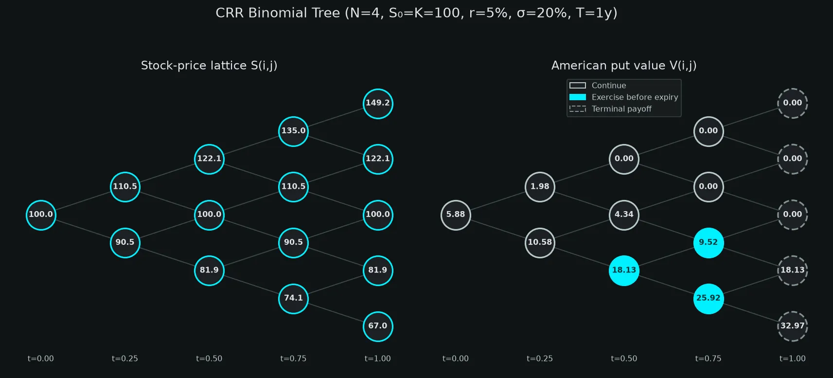
Here is the vectorised Python implementation:

def crr_american_put(S0, K, r, sigma, T, n_steps):
    """CRR binomial tree for an American put. O(n²) time, O(n) memory."""
    dt   = T / n_steps
    u    = np.exp(sigma * np.sqrt(dt))
    d    = 1 / u
    p    = (np.exp(r * dt) - d) / (u - d)
    disc = np.exp(-r * dt)

    j   = np.arange(n_steps + 1)
    S_T = S0 * u**(n_steps - j) * d**j
    V   = np.maximum(K - S_T, 0.0)            # terminal payoffs

    for i in range(n_steps - 1, -1, -1):
        j2  = np.arange(i + 1)
        S_t = S0 * u**(i - j2) * d**j2
        V   = disc * (p * V[:-1] + (1 - p) * V[1:])   # roll back
        V   = np.maximum(V, np.maximum(K - S_t, 0.0))  # early exercise check

    return float(V[0])

Running this for the standard at-the-money case ( $S_{0} = K = 100$ , $r = 5%$ , $σ = 20%$ , $T = 1$ year):

CRR(1000) American put: 6.0896
High-step parity-pair ref: 6.0904
BS European put:        5.5735
Early exercise premium: ≈ 0.517

The Convergence Problem

Increasing $N$ should improve accuracy. For CRR, it does — but not smoothly. The price oscillates above and below the true value as $N$ increases.

The oscillation has a structural cause. At expiry, the position of the strike relative to the terminal lattice changes with the parity and size of $N$ , altering how the kink in the payoff is sampled. Before expiry, the discrete exercise boundary also moves in one-node increments. These payoff-alignment and boundary-discretisation errors propagate backward through the tree and create the familiar odd-even bias.

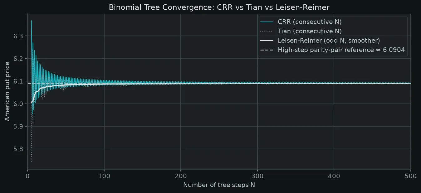
Convergence chart using consecutive step counts for CRR and Tian and odd step counts for Leisen-Reimer. CRR shows an odd-even sawtooth while Leisen-Reimer approaches the reference more smoothly. — Convergence comparison: consecutive CRR refinements reveal the odd-even sawtooth; Tian still oscillates; Leisen-Reimer uses odd N and converges more smoothly. Parameters: S₀=K=100, r=5%, σ=20%, T=1y.

The oscillation means that a larger CRR step count is not guaranteed to beat the immediately preceding count. Accuracy should therefore be measured against a converged benchmark and, when possible, checked across both parity subsequences. For the example above, CRR(1000) is about $0.0008$ from a high-step parity-pair benchmark—roughly 1.3 basis points relative to the option value, or 0.08 cents per share.

Improved Tree Methods

Tian (1993): Moment Matching

Tian's approach chooses $u$ , $d$ , and $p$ to match the first three moments of the lognormal stock-price distribution over each interval $Δ t$ : mean, variance, and skewness. The parametrisation uses:

$u = \frac{1}{2} M V^{2} (V^{2} + 1 + V^{4} + 2 V^{2} - 3), V^{2} = e^{σ^{2} Δ t}, M = e^{r Δ t}$

$d = \frac{1}{2} M V^{2} (V^{2} + 1 - V^{4} + 2 V^{2} - 3)$

This reduces the oscillation compared to CRR, but does not eliminate it entirely.

Leisen-Reimer (1996): Node Placement

Leisen and Reimer took a different approach. Instead of matching moments, they asked: what node placement makes the binomial distribution align exactly with the Black-Scholes probabilities?

They used the Peizer-Pratt inversion formula—which maps normal quantiles to binomial probabilities—to position nodes so that the terminal distribution of the tree closely matches the lognormal:

$p = h (d_{2}), p^{'} = h (d_{1})$

where $h$ is the Peizer-Pratt Method 2 inversion and $d_{1}$ , $d_{2}$ are the standard Black-Scholes parameters. Here $p$ is the risk-neutral up-probability used during rollback; $p^{'}$ is an auxiliary probability used to derive the up and down factors.

def leisen_reimer_american_put(S0, K, r, sigma, T, n_steps):
    """Leisen-Reimer (1996) — Peizer-Pratt Method 2 node placement."""
    if n_steps % 2 == 0:
        n_steps += 1   # LR requires an odd number of steps

    def peizer_pratt_2(z, n):
        return 0.5 + np.sign(z) * np.sqrt(
            0.25 - 0.25 * np.exp(
                -(z / (n + 1/3 + 0.1/(n+1)))**2 * (n + 1/6)))

    dt = T / n_steps
    d1 = (np.log(S0/K) + (r + 0.5*sigma**2)*T) / (sigma*np.sqrt(T))
    d2 = d1 - sigma*np.sqrt(T)
    p_prime = peizer_pratt_2(d1, n_steps)
    p       = peizer_pratt_2(d2, n_steps)
    u       = np.exp(r*dt) * p_prime / p
    d       = (np.exp(r*dt) - p*u) / (1 - p)
    disc = np.exp(-r*dt)
    # ... same backward induction using p

The LR tree converges much more smoothly, but not necessarily monotonically at every refinement. For this contract, LR(51) is about $0.0068$ from the high-step benchmark—comfortably within one cent, but about 11 relative basis points. That distinction matters: a cent of absolute option value is not the same accuracy target as one basis point of relative error.

Because all three rollback algorithms take $O (N^{2})$ work, reducing the step count can still produce a large speedup. The original Leisen-Reimer study reports that its new trees reached the same accuracy about ten times faster on average for American options; the exact ratio depends on the contract, implementation, and error definition.

Leisen-Reimer substantially smooths lattice convergence, but accuracy still needs a clearly defined error unit and a contract-specific benchmark.

The Free Boundary from a Tree

The tree not only prices the option — it also identifies the free boundary at each time step. At step $i$ , the boundary is the highest stock price at which the exercise constraint binds:

$S^{*} (t_{i}) = max {S_{i, j} : K - S_{i, j} > e^{- r Δ t} [p V_{i + 1, j} + (1 - p) V_{i + 1, j + 1}]}$

In other words: the highest stock price node where the tree chose early exercise.

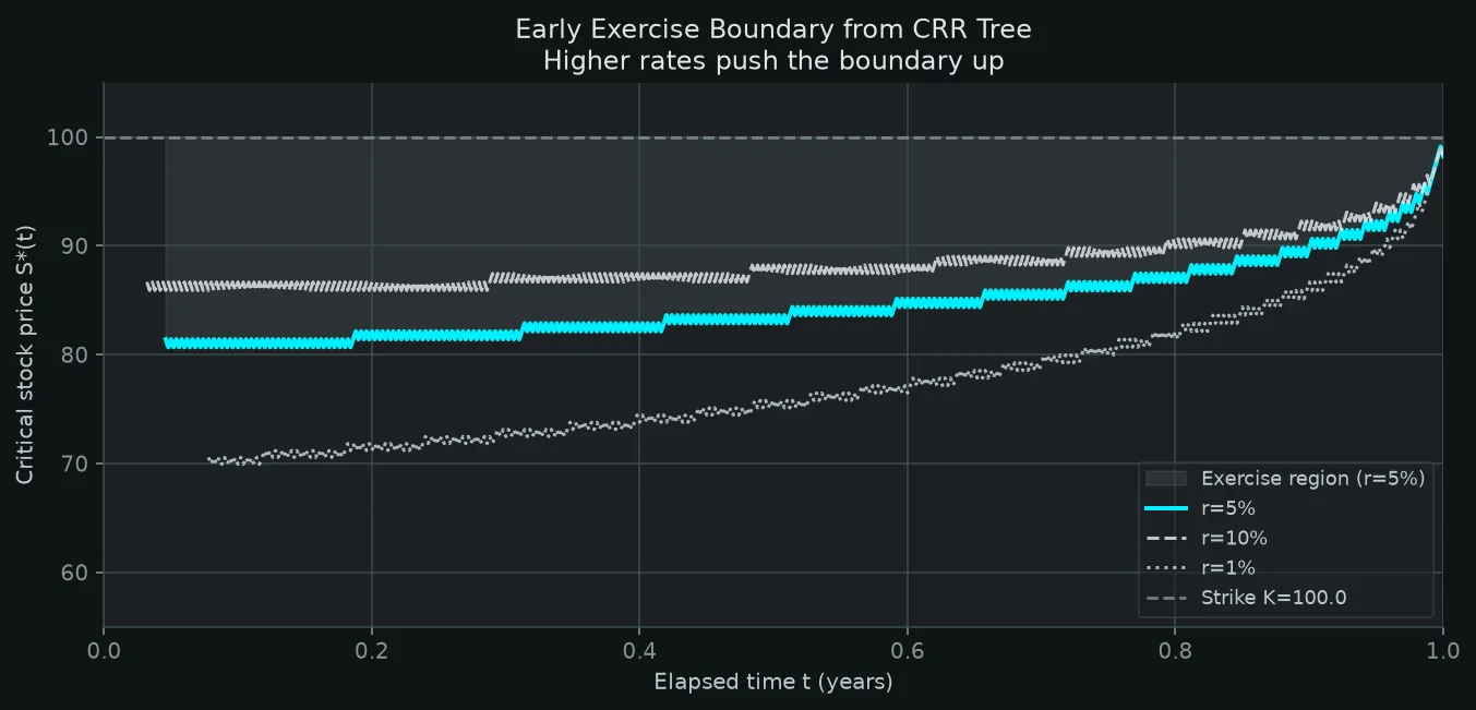
Free exercise boundary extracted from a CRR tree against elapsed time at three interest rates. The boundary rises toward K as maturity approaches, and higher rates produce a larger exercise region. — Free boundary from CRR(500) at three interest rates. Higher rates push the boundary up — more stock price range triggers early exercise. S₀=K=100, σ=20%, T=1y.

The boundary is not exact—it inherits the node granularity of the tree. A 500-step CRR tree has 501 time levels, including today and maturity, at intervals of 0.002 years. Some early levels may contain no exercise node because the finite lattice has not yet reached the exercise region. Where the boundary is observed, the dense CRR grid provides a useful approximation to the continuous $S^{*} (t)$ .

When to Use Trees

Binomial trees work well for:

1D vanilla American options — puts and calls with dividends
Simple barriers — monitored barriers can be enforced at lattice nodes, with care around barrier alignment
Quick indicative pricing — modest trees can deliver cent-level accuracy for many contracts
Teaching and intuition — the backward induction structure is transparent

They become awkward for:

Strongly path-dependent payoffs — Asian and lookback options require an augmented state, which weakens or destroys recombination
Multiple underlyings — a recombining two-asset lattice grows polynomially in $N$ , but the state count suffers from the curse of dimensionality and grows exponentially with the number of risk factors
Complex vol surfaces — a constant-volatility tree cannot fit a full surface; implied or local-volatility trees require additional calibration and stability checks

For many 1D problems that need high accuracy, a finite-difference method such as Crank-Nicolson (Part 3) is competitive and often easier to refine systematically. For multi-dimensional early-exercise problems, Longstaff-Schwartz Monte Carlo (Part 4) is a common choice.

Companion Notebook

The Python notebook for this post is available for download: american-options-binomial-trees.ipynb. It includes:

CRR, Tian, and Leisen-Reimer implementations
Convergence study (N=5 to N=500)
Free boundary extraction at multiple rate levels
Exercises for trinomial trees and timing comparisons

Previous Posts in This Thread

The American Option Problem: Why Early Exercise Has No Closed Form covers optimal stopping theory, the free boundary, and the LCP formulation.
Monte Carlo Option Pricing: When Closed Forms Stop Helping introduces path simulation and European MC pricing.

References

John C. Cox, Stephen A. Ross, and Mark Rubinstein, "Option Pricing: A Simplified Approach", Journal of Financial Economics, 1979.
Yisong Tian, "A Modified Lattice Approach to Option Pricing", Journal of Futures Markets, 1993.
Dietmar Leisen and Matthias Reimer, "Binomial Models for Option Valuation — Examining and Improving Convergence", Applied Mathematical Finance, 1996.

Get in Touch

Building option pricing models or studying binomial tree methods?

Connect with me:

📧 Email: [email protected]
🐦 Twitter/X: @TheDataGuyPro
💼 LinkedIn: Muhammad Afzaal
💻 GitHub: @mafzaal
🎥 YouTube: @TheDataGuyPro
🎧 Podcast: TheDataGuy Show

Whether you're implementing trees from scratch or comparing convergence methods, I'd love to hear from you!

Contents