Finite Differences and PSOR: Solving the American Put PDE

How do you turn “exercise whenever it is optimal” into equations a computer can solve? The previous post answered with backward induction on a binomial tree. Here we take the continuous-time route: start from the Black-Scholes PDE, convert early exercise into an inequality constraint, and solve the resulting system on a grid.

Finite difference methods take a different approach. Instead of discretising the stochastic process, they discretise the partial differential equation directly. The result is a system of equations on a spatial grid — and for American options, that system has a twist: it must simultaneously satisfy the PDE and the exercise constraint.

That twist is the linear complementarity problem. This post develops it one layer at a time: first the economic intuition, then the finite-difference stencil, then the Projected SOR (PSOR) iteration. By the end, you should be able to explain every term in the implementation, diagnose convergence, and recover the early-exercise boundary from the solution.

This is Part 3 of the American Options sub-series.

Contents

---

From Tree to Grid

Assume a non-dividend-paying stock follows the Black-Scholes model with constant non-negative interest rate $r$ and volatility $\sigma$. The PDE for a European option is:

$$\frac{\partial V}{\partial t}+\frac{1}{2}{\sigma }^2{S}^2\frac{{\partial }^{2}V}{\partial S^2}+rS\frac{\partial V}{\partial S}-rV=0$$

For a European option, this PDE holds on the entire domain $(0,\infty )\times [0,T]$ with a fixed terminal condition $V(S,T)=\max (K-S,0)$.

For an American put, the holder can stop the contract at any time and receive the intrinsic value

$$\Psi (S)=\max (K-S,0).$$

This creates two non-negotiable conditions. First, the option can never be worth less than immediate exercise, so $V\ge \Psi$. Second, in any region where waiting is optimal, the usual Black-Scholes PDE must hold: otherwise a locally riskless arbitrage would remain.

Where exercise is optimal, the PDE need not hold with equality. The option has been pinned to the obstacle $\Psi$, and waiting must not be more valuable than stopping. It is useful to define the calendar-time PDE residual

$$R(V)=-\left(V_t+\frac{1}{2}{\sigma }^2{S}^2{V}_{SS}+rS{V}_S-rV\right).$$

Then $R(V)\ge 0$, $V-\Psi \ge 0$, and at least one of them must be zero at every point. That gives the linear complementarity problem (LCP):

$$\min \left(-\frac{\partial V}{\partial t}-\frac{1}{2}{\sigma }^2{S}^2\frac{{\partial }^{2}V}{\partial S^2}-rS\frac{\partial V}{\partial S}+rV,V-\Psi \right)=0$$

The minimum is taken pointwise. Equivalently,

$$R(V)\ge 0,V-\Psi \ge 0,R(V)(V-\Psi )=0.$$

The last equation is the complementarity condition. It says that the PDE residual and the value-above-exercise gap cannot both be strictly positive:

For a quick sign check, consider the in-the-money exercise payoff $V=K-S$. It has $V_t=0$, $V_S=-1$, and $V_{SS}=0$, so $R(V)=rK\ge 0$. Economically, waiting to receive $K$ sacrifices interest on the strike; that is precisely why early exercise can be valuable for a put when rates are positive.

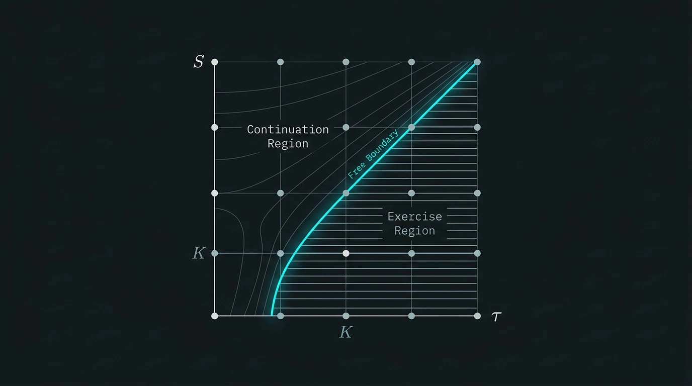
The boundary between the two regions is the unknown free boundary $S^{\ast }(t)$. Under the usual regularity assumptions it satisfies value matching and smooth pasting:

$$V(S^{\ast }(t),t)=K-S^{\ast }(t),V_S(S^{\ast }(t),t)=-1.$$

We will not impose $S^{\ast }(t)$ on the grid. The LCP will decide which nodes exercise, and the boundary will emerge from those decisions.

Why Switch to Time to Maturity?

Pricing runs backward in calendar time: the payoff is known at $t=T$, but the desired price is at $t=0$. Define time to maturity $\tau =T-t$ and $U(S,\tau )=V(S,T-\tau )$. Since $V_t=-U_{\tau }$, the continuation PDE becomes

$$ U_\tau=\mathcal L U,\qquad \mathcal LU=\frac{1}{2}\sigma^2S^2U_{SS}+rSU_S-rU.$$

Now the computation moves forward in $\tau$ from the known initial condition $U(S,0)=\Psi (S)$ to $U(S,T)=V(S,0)$. The obstacle form becomes

$$\min \left(U_{\tau }-\mathcal{L}U,U-\Psi \right)=0.$$

---

Crank-Nicolson Discretisation

Finite difference methods replace the continuous $(S,\tau )$ domain with a finite set of nodes. Choose a large but finite $S_{\max }$ and define:

• $S_i=i\cdot \Delta S$ for $i=0,1,\dots ,N_S$ with $\Delta S=S_{\max }/N_S$
• ${\tau }_m=m\cdot \Delta \tau$ for $m=0,1,\dots ,N_t$, where ${\tau }_0=0$ is maturity and ${\tau }_{N_t}=T$ is today
• $U_i^m=V(S_i,T-{\tau }_m)$, with $U_i^0=\Psi (S_i)$

The stock-price domain has been truncated from $[0,\infty )$ to $[0,S_{\max }]$. This introduces a domain error that is separate from the grid-spacing error; later we will vary $S_{\max }$ and $N_S$ independently.

At an interior node, use the three-point central differences

$$\frac{{\partial }^{2}U}{\partial S^2}{|}_{S_i}\approx \frac{U_{i+1}-2U_i+U_{i-1}}{\Delta S^2},\frac{\partial U}{\partial S}{|}_{S_i}\approx \frac{U_{i+1}-U_{i-1}}{2\Delta S}$$

Substituting them into $\mathcal{L}$ gives a three-node stencil:

$$L_h{U}_i={\alpha }_i{U}_{i-1}+{\beta }_i{U}_i+{\gamma }_i{U}_{i+1},$$

where

$${\alpha }_i=\frac{1}{2}\frac{{\sigma }^2{S}_i^2}{\Delta S^2}-\frac{r{S}_i}{2\Delta S},{\beta }_i=-\frac{{\sigma }^2{S}_i^2}{\Delta S^2}-r,{\gamma }_i=\frac{1}{2}\frac{{\sigma }^2{S}_i^2}{\Delta S^2}+\frac{r{S}_i}{2\Delta S}.$$

This formula is the bridge from the differential operator to a matrix: ${\alpha }_i$, ${\beta }_i$, and ${\gamma }_i$ become the lower, main, and upper diagonals.

Why Crank-Nicolson?

Forward Euler would evaluate $L_{h}U$ only at the known layer $m$. Backward Euler would evaluate it only at the unknown layer $m+1$. Crank-Nicolson averages the two:

$$\frac{U_i^{m+1}-U_i^m}{\Delta \tau }=\frac{1}{2}\left(L_h{U}_i^m+L_h{U}_i^{m+1}\right).$$

It is implicit, so every new node depends on its neighbours at the new layer. For smooth solutions it is second-order accurate in both $\Delta S$ and $\Delta \tau$, while avoiding the severe time-step restriction of an explicit scheme. Rearranging the interior-node equation gives

$$-a_i{U}_{i-1}^{m+1}+b_i{U}_i^{m+1}-c_i{U}_{i+1}^{m+1}=a_i{U}_{i-1}^m+(2-b_i)U_i^m+c_i{U}_{i+1}^m,$$

with:

$$a_i=\frac{\Delta \tau }{4}\left(\frac{{\sigma }^2{S}_i^2}{\Delta S^2}-\frac{r{S}_i}{\Delta S}\right),b_i=1+\frac{\Delta \tau }{2}\left(\frac{{\sigma }^2{S}_i^2}{\Delta S^2}+r\right),c_i=\frac{\Delta \tau }{4}\left(\frac{{\sigma }^2{S}_i^2}{\Delta S^2}+\frac{r{S}_i}{\Delta S}\right).$$

On the uniform grid $S_i=i\Delta S$, these simplify to

$$a_i=\frac{\Delta \tau }{4}({\sigma }^2{i}^2-ri),b_i=1+\frac{\Delta \tau }{2}({\sigma }^2{i}^2+r),c_i=\frac{\Delta \tau }{4}({\sigma }^2{i}^2+ri).$$

That simplified form is useful for checking an implementation, but the $S_i$ form generalises more naturally to non-uniform coordinates and other models.

From the Stencil to a Matrix

For a European option, this is a tridiagonal linear system, solvable with the Thomas algorithm in $O(N_S)$ work per time step.

For the interior unknown vector $U^{m+1}=(U_1^{m+1},\dots ,U_{N_S-1}^{m+1}{)}^{\top }$, the matrix has the structure

$$A=\left[\begin{array}{cccc}{b}_1& -c_1& & \\ -a_2& b_2& -c_2& \\ & \ddots & \ddots & \ddots \\ & & -a_{N_S-1}& b_{N_S-1}\end{array}\right]$$

The vector $d^m$ contains the right-hand side built from the known layer $U^m$ plus any boundary contributions. For an American put we use

$$U_0^m=K,U_{N_S}^m=0.$$

The old left boundary already appears in $a_1{U}_0^m$ on the explicit side. Moving the new left-boundary term $-a_1{U}_0^{m+1}$ off the matrix adds another $a_{1}K$ to the first entry of $d^m$. The upper boundary contributes zero under the far-field approximation.

For an American option, let $A$ be the tridiagonal matrix on the left and $d^m$ the right-hand side after boundary terms are included. Each new layer must satisfy the discrete LCP

$$A{U}^{m+1}-d^m\ge 0,U^{m+1}-\Psi \ge 0,$$

$${\left(A{U}^{m+1}-d^m\right)}_i\left(U_i^{m+1}-{\Psi }_i\right)=0\text{for every interior node }i.$$

A plain tridiagonal solve enforces $A{U}^{m+1}=d^m$ everywhere, including nodes where exercise should bind. Clipping that solution to the payoff only once is also insufficient: changing one node changes the neighbouring matrix equations. The linear equations and the obstacle constraint must be solved together.

---

Projected SOR (PSOR)

PSOR is easiest to understand as “solve locally, relax, then enforce the contract.” During sweep $k+1$, the algorithm visits the interior nodes from left to right.

First compute the Gauss-Seidel value that would satisfy row $i$ of the linear system. It uses the already-updated left neighbour and the not-yet-updated right neighbour:

$${\hat{U}}_i^{(k+1)}=\frac{1}{b_i}\left(d_i^m+a_i{U}_{i-1}^{(k+1)}+c_i{U}_{i+1}^{(k)}\right).$$

Then blend that candidate with the current iterate:

$$U_{i,\mathrm{SOR}}^{(k+1)}=U_i^{(k)}+\omega \left({\hat{U}}_i^{(k+1)}-U_i^{(k)}\right).$$

Finally project onto the exercise constraint:

$$U_i^{(k+1)}=\max \left(U_{i,\mathrm{SOR}}^{(k+1)},{\Psi }_i\right).$$

The word projected refers exactly to this last maximum. The update can never finish below the payoff. Repeating the sweep lets the projected nodes and their neighbours adjust to one another until both the matrix inequality and the obstacle are satisfied.

The relaxation parameter controls how far the iteration moves:

• $0<\omega <1$: under-relaxation; more cautious, usually slower.
• $\omega =1$: projected Gauss-Seidel.
• $1<\omega <2$: over-relaxation; often faster when tuned well.

One Complete Time Step

At each new time-to-maturity layer, the solver performs the same sequence:

1. Treat $U^m$ as known and build $d^m$.
2. Start the unknown layer from $U^m$; this warm start is usually close because adjacent time levels differ only slightly.
3. Sweep through the stock-price nodes with the SOR update and payoff projection.
4. Repeat until the iterate change and the complementarity residual are both small.
5. Store the converged layer as $U^{m+1}$ and advance in $\tau$.

For a discrete candidate $x$, define

$$w=Ax-d^m,z=x-\Psi .$$

The LCP requires $w\ge 0$, $z\ge 0$, and $\min (w_i,z_i)=0$ at every node. A compact numerical check is therefore

$$R_{\mathrm{LCP}}(x)={\Vert \min (Ax-d^m,x-\Psi )\Vert }_{\infty },$$

where the minimum is componentwise. Unlike iterate change alone, this tests the equations we actually want to solve. The implementation below requires both checks and raises an error if PSOR reaches its iteration cap.

import numpy as np


def cn_psor_american_put(S0, K, r, sigma, T,
                         N_S=100, N_t=100, S_max_factor=3.0,
                         omega=1.2, psor_iters=500, tol=1e-8):
    if S0 <= 0.0 or K <= 0.0 or sigma <= 0.0 or T <= 0.0 or r < 0.0:
        raise ValueError("Use S0, K, sigma, T > 0 and r >= 0")
    if N_S < 3 or N_t < 1 or S_max_factor <= 1.0:
        raise ValueError("Use N_S >= 3, N_t >= 1, S_max_factor > 1")
    if not (0.0 < omega < 2.0):
        raise ValueError("omega must be between 0 and 2")

    S_max = S_max_factor * max(S0, K)
    dS    = S_max / N_S
    dt    = T / N_t
    S     = np.linspace(0, S_max, N_S + 1)
    n_int = N_S - 1

    def payoff(S_):
        return np.maximum(K - S_, 0.0)

    V = payoff(S).copy()  # tau=0: payoff at maturity
    S_int = np.arange(1, N_S, dtype=float) * dS

    # Crank-Nicolson coefficients from the derivation above
    a = 0.25*dt*(sigma**2*S_int**2/dS**2 - r*S_int/dS)
    b = 1.0 + 0.5*dt*(sigma**2*S_int**2/dS**2 + r)
    c = 0.25*dt*(sigma**2*S_int**2/dS**2 + r*S_int/dS)

    for _ in range(N_t):
        V_old = V.copy()
        rhs = a*V_old[:-2] + (2.0-b)*V_old[1:-1] + c*V_old[2:]
        rhs[0] += a[0]*K   # implicit contribution from V(0, tau)=K

        obstacle = payoff(S_int)
        V_int = V_old[1:-1].copy()  # warm start from previous layer

        def lcp_residual(x):
            # Apply the interior tridiagonal matrix A. Boundary terms
            # have already been moved into rhs.
            Ax = b*x.copy()
            Ax[1:] -= a[1:]*x[:-1]
            Ax[:-1] -= c[:-1]*x[1:]
            return float(np.max(np.abs(np.minimum(Ax-rhs, x-obstacle))))

        converged = False
        for _ in range(psor_iters):
            max_chg = 0.0
            for k in range(n_int):
                left_  = V_int[k-1] if k > 0 else 0.0  # a[0]*K is already in rhs[0]
                right_ = V_int[k+1] if k < n_int-1 else 0.0
                V_sor  = (rhs[k] + a[k]*left_ + c[k]*right_) / b[k]
                V_upd  = V_int[k] + omega*(V_sor - V_int[k])
                V_upd  = max(V_upd, obstacle[k])   # projection step
                max_chg = max(max_chg, abs(V_upd - V_int[k]))
                V_int[k] = V_upd
            if max_chg < tol and lcp_residual(V_int) < tol:
                converged = True
                break

        if not converged:
            raise RuntimeError("PSOR failed to converge")

        V[0] = K
        V[-1] = 0.0
        V[1:-1] = V_int

    return float(np.interp(S0, S, V))

For $S_0=K=100$, $r=5\%$, $\sigma =20\%$, and $T=1$, the $100\times 100$ grid returns about $6.0997$. The corresponding European Black-Scholes put is about $5.5735$, so the roughly $0.53$ difference is the early-exercise premium at this grid resolution. This gives a useful sanity chain:

$$V_{\text{American put}}\ge V_{\text{European put}}\ge \max (K{e}^{-rT}-S_0,0),$$

and, independently, $V_{\text{American put}}\ge \max (K-S_0,0)$ because the American holder can exercise immediately.

The boundary conditions are:

• $S=0$: an American put worth $K$ immediately (exercise now, stock can never recover from zero) → $V(0,t)=K$
• $S=S_{\max }$: an approximation to the far-field condition $V(S,t)\to 0$ as $S\to \infty$

The upper boundary is a truncation, not an exact condition at arbitrary finite $S_{\max }$. Increase $S_{\max }$ and refine the grid to confirm that truncation error is negligible for the contract being priced.

Central differencing also needs care when drift dominates diffusion near the left edge: the coefficient $a_i$ can become negative, so the discrete operator need not be monotone. Log-price coordinates, non-uniform grids, or an upwind/fitted treatment of the first derivative are common remedies when this affects the contract or parameter regime.

What the Code Is Really Solving

The outer loop evolves the option from maturity to today. The inner PSOR loop resolves the exercise decision at one time layer. Those are different convergence problems:

• Increasing $N_t$ reduces time-discretisation error.
• Increasing $N_S$ reduces spatial-discretisation error.
• Increasing $S_{\max }$ checks domain-truncation error.
• Tightening tol reduces algebraic error from the iterative LCP solve.

Changing all four at once can hide the source of an error. A disciplined convergence study varies one control at a time.

---

The Option Value Surface

If each time layer is retained instead of overwritten, CN-PSOR gives the option value surface $V(S,t)$ as well as today’s price.

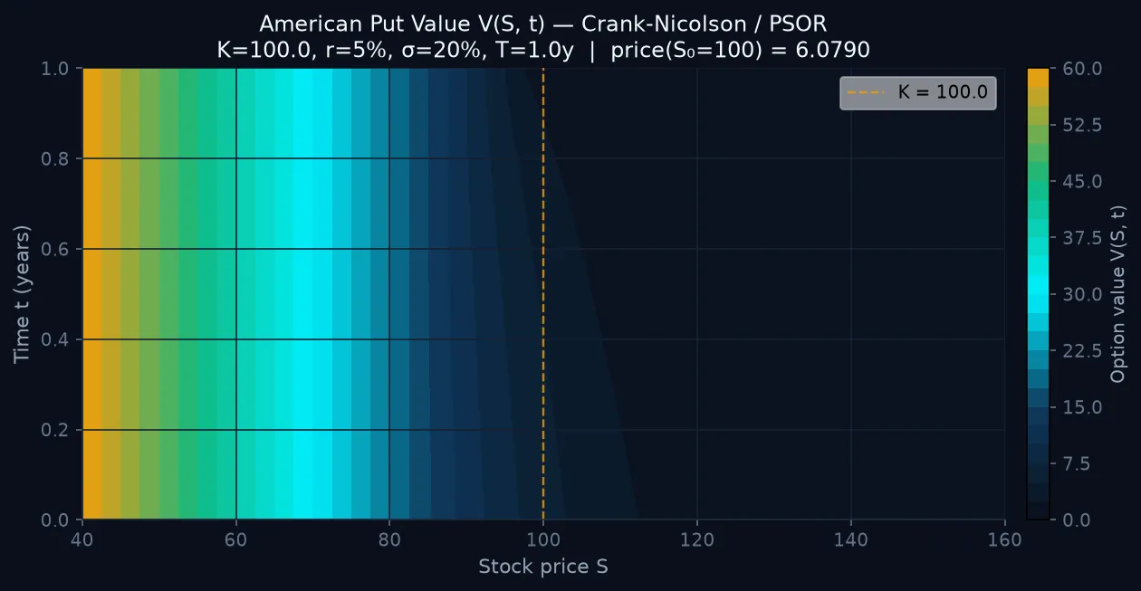
The two regimes are identified by the gap $V-\Psi$:

• Continuation region (to the right of the boundary before maturity): $V>\Psi$, so the option has positive continuation value.
• Exercise region (to the left of the boundary): $V=K-S$, so the surface is linear in $S$.

At maturity, $V=\Psi$ everywhere; “exercise” versus “continue” is no longer a meaningful choice.

---

The Free Boundary from PSOR

The free boundary is extracted from the PSOR solution by identifying, at each time step, the largest in-the-money node where the exercise constraint binds. Numerically, use a small gap tolerance and require $\Psi (S_i)>0$:

$$S^{\ast }(t_m)\approx \max \{S_i:\Psi (S_i)>0\text{and}{V}_i^m-\Psi (S_i)\le {\epsilon }_{\text{boundary}}\}.$$

The in-the-money test matters: far out-of-the-money nodes can have both payoff and computed value close to zero, but they are not part of the put’s exercise region.

Why take the largest exercise node? For a vanilla put, exercise occurs at low stock prices. At a fixed time, the grid typically looks like

$$\underset{S_i\le S^{\ast }(t)}{\underbrace{\text{exercise},\dots ,\text{exercise}}}|\underset{S_i>S^{\ast }(t)}{\underbrace{\text{continue},\dots ,\text{continue}}}.$$

The rightmost exercise node is therefore the node-level estimate of $S^{\ast }(t)$. Because it can only land on grid points, the extracted curve is stair-stepped. A finer grid reduces those jumps; interpolation using the obstacle gap or the smooth-pasting condition can produce a sub-grid estimate, but it does not replace a convergence study.

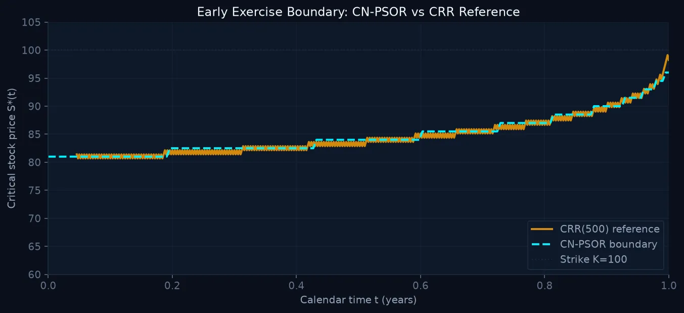
The CN-PSOR boundary closely tracks the CRR(500) comparator. Small differences arise because both methods discretise the boundary on different node sets. Agreement between two discretisations is a useful cross-check, not proof that either boundary is exact.

The shape also has an economic interpretation. With little time remaining, the critical price rises toward the strike because there is less optionality left to preserve. Farther from maturity, the holder is willing to tolerate a lower stock price before exercising because the remaining time value is larger.

---

Grid Convergence

For a sufficiently smooth solution, central spatial differences and Crank-Nicolson have formal truncation error $O(\Delta S^2+\Delta {\tau }^2)$. An American put is less tidy: the payoff has a kink, the free boundary reduces regularity, the domain is truncated, and the PSOR tolerance adds algebraic error. Raw grid errors can therefore be non-monotone even when the asymptotic error envelope is close to second order.

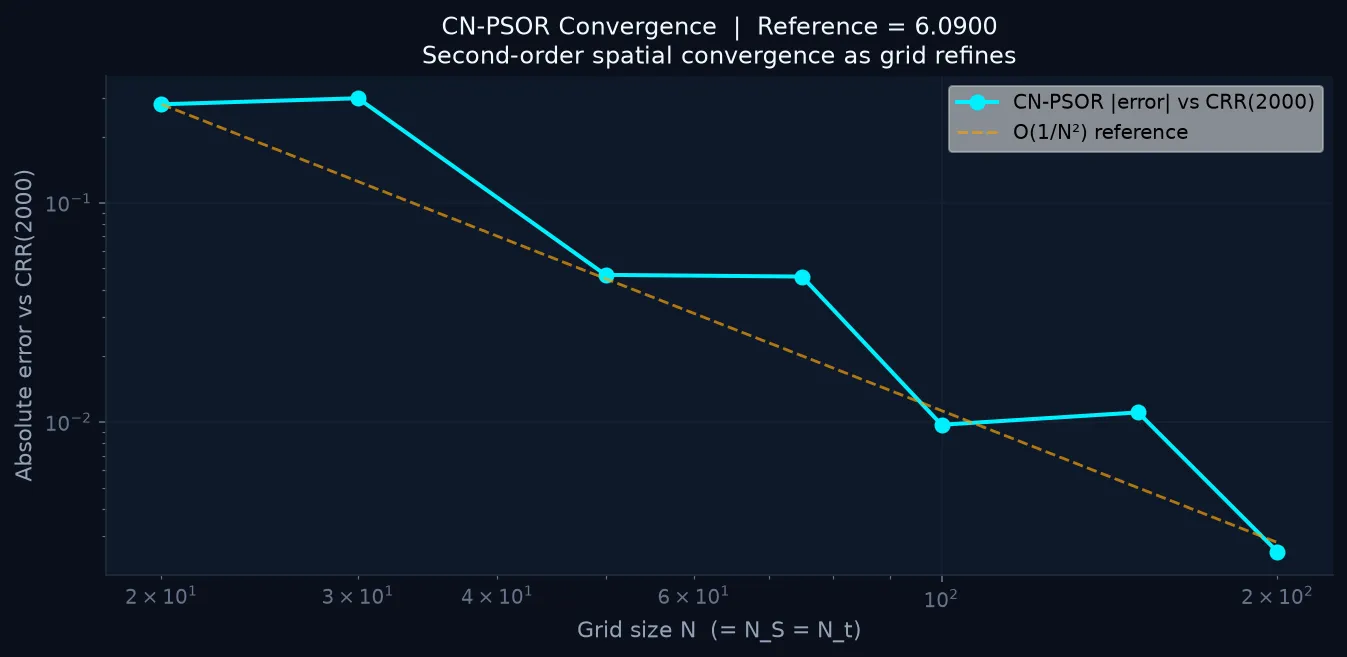
The computed values behind the chart reproduce as follows. “Error” means absolute difference from CRR(2000), not error against an exact American-option value:

The comparison table for the standard at-the-money American put:

The aligned 50→100→200 refinement sequence is consistent with roughly second-order decay, but the omitted 30, 75, and 150 grids oscillate rather than decrease monotonically. For more reliable convergence studies, use a better-converged independent benchmark, verify $S_{\max }$ separately, and consider Rannacher startup steps (a few backward-Euler substeps before Crank-Nicolson) to damp payoff-kink oscillations.

Separate the Four Error Sources

A reported “finite-difference error” is usually a mixture:

This separation matters. For example, increasing $N_S$ while holding S_max_factor fixed reduces $\Delta S$, but increasing S_max_factor while holding $N_S$ fixed makes $\Delta S$ larger. The second change improves the far boundary and worsens local resolution at the same time.

Numerical Sanity Checks

A solver can converge numerically and still solve the wrong discretised problem. For a vanilla American put, check these invariants:

• Obstacle: $V_i^m\ge {\Psi }_i$ at every node.
• Complementarity: $\Vert \min (AV-d,V-\Psi ){\Vert }_{\infty }$ is below tolerance at every time layer.
• Bounds: $\Psi (S)\le V(S,t)\le K$ for $r\ge 0$.
• Shape in stock price: the put value should be non-increasing and normally convex in $S$.
• European comparison: the American put should not be worth less than the otherwise identical European put.
• Boundary policy: in-the-money nodes should form one contiguous exercise region at the low-$S$ end for this vanilla one-factor case.
• Refinement: the price should stabilise as the domain, spatial grid, time grid, and PSOR tolerance are refined separately.

These checks catch common bugs such as a reversed time direction, a missing implicit boundary contribution, the wrong sign on $a_i$ or $c_i$, and false exercise detection at zero-payoff nodes.

---

Choosing the Over-Relaxation Parameter

The parameter $\omega$ controls the SOR convergence rate. For $\omega =1$, the algorithm reduces to Gauss-Seidel (standard sequential updates). For $\omega >1$, updates are "over-relaxed" — each iterate moves further in the direction of the correction.

The optimal $\omega$ depends on the iteration matrix and therefore on the grid, time step, and model coefficients. Values around $1.2$ – $1.5$ are reasonable experiments for this example, not universal defaults. The usual SOR convergence theory does not extend to $\omega \ge 2$, and such choices typically diverge.

In practice, test several values against the same complementarity-residual tolerance and compare total solve time—not just the iteration count.

---

When to Use Finite Differences

FDM with CN-PSOR is a useful baseline and a practical approach for one-factor American option pricing:

• Structure: each PSOR sweep is $O(N_S)$ because the matrix is tridiagonal
• Accuracy controls: spatial, temporal, truncation, and iterative errors can be tested separately
• Flexibility: local-volatility coefficients, dividends, and many early-exercise payoff variants fit the same PDE/LCP framework
• Free boundary: can be extracted from the converged grid for diagnostics and exercise-policy analysis

PSOR is not automatically the fastest production LCP solver. Direct projected methods, penalty or policy-iteration schemes, and operator splitting can be materially faster for some models and grids.

FDM becomes impractical for:

• More than two underlying assets: the curse of dimensionality makes the grid exponentially large
• Path-dependent payoffs: the PDE framework requires augmenting the state space, which quickly becomes intractable
• High-dimensional models: interest rate models with many factors, credit models with multiple obligors

For those cases, Longstaff-Schwartz Monte Carlo (Part 4) is a common alternative, especially when simulation is already natural for the model.

---

Companion Notebook

The Python notebook for this post is available for download: american-options-finite-difference.ipynb. It includes:

• Full CN-PSOR implementation with boundary extraction
• Option value surface visualisation
• Free boundary comparison against CRR reference
• Grid convergence study
• Exercises for the penalty method and omega tuning

---

Previous Posts in This Thread

• Binomial Trees for American Puts implements CRR and Leisen-Reimer trees and explains the convergence oscillation problem.
• The American Option Problem: Why Early Exercise Has No Closed Form establishes the theory.

---

References

• Michael Brennan and Eduardo Schwartz, "The Valuation of American Put Options", Journal of Finance, 1977.
• John Crank and Phyllis Nicolson, "A Practical Method for Numerical Evaluation of Solutions of Partial Differential Equations of the Heat-Conduction Type", Proceedings of the Cambridge Philosophical Society, 1947.
• Liming Feng, Vadim Linetsky, José Luis Morales, and Jorge Nocedal, "On the Solution of Complementarity Problems Arising in American Options Pricing", Optimization Methods and Software, 2011.
• Samuli Ikonen and Jari Toivanen, "Operator Splitting Methods for American Option Pricing", Applied Mathematics Letters, 2004.
• Paul Wilmott, Jeff Dewynne, and Sam Howison, Option Pricing: Mathematical Models and Computation, Oxford Financial Press, 1993.
• Daniel Duffy, Finite Difference Methods in Financial Engineering: A Partial Differential Equation Approach, Wiley, 2006.

---

Get in Touch

Working on PDE methods for derivatives, or comparing FDM and Monte Carlo for American options?

Connect with me:

• 📧 Email: [email protected]
• 🐦 Twitter/X: @TheDataGuyPro
• 💼 LinkedIn: Muhammad Afzaal
• 💻 GitHub: @mafzaal
• 🎥 YouTube: @TheDataGuyPro
• 🎧 Podcast: TheDataGuy Show

Whether you're implementing production pricing engines or exploring numerical PDE methods, I'd love to hear from you!