Value at Risk in Python: Rolling Volatility, EWMA, and Breach Testing
In the late 1980s, Dennis Weatherstone — then a senior executive at J.P. Morgan and later its chairman — had a problem.
He was running one of the largest trading operations in the world and he could not get a straight answer to a simple question:
How much money could we lose tomorrow?
Not across all possible scenarios. Not in the most catastrophic case imaginable. Just: at the end of a normal bad day, how bad could it be?
As the origin story is usually told, he asked for a one-page risk report delivered after the market close. Its headline number estimated the potential loss over the next 24 hours at 95% confidence. The report became known as the 4:15 report.
The result — after years of internal development by J.P. Morgan's researchers — was RiskMetrics, released publicly in October 1994.
The methodology that underpinned the number was called Value at Risk.
VaR spread quickly through banks and trading desks. The Basel Committee's 1996 Market Risk Amendment permitted approved banks to use internal VaR models for market-risk capital, and the framework was later incorporated into Basel II.
Then 2008 happened.
VaR measures how bad a bad day looks. It says nothing about how bad the worst day actually gets.
This is the sixth post in the Randomness to Risk series. The earlier posts built the machinery for pricing derivatives — GBM, Black-Scholes, Monte Carlo, American options. This post pivots from pricing to risk measurement. The question changes from "what is this worth?" to "how much could we lose?"
This is educational research. Not investment advice, and not a substitute for understanding your own portfolio's risk properly.
Contents
What VaR Actually Says
Value at Risk is a quantile of the loss distribution.
At confidence level and horizon , VaR is the smallest threshold such that the probability of a loss no greater than is at least :
For a continuous loss distribution, this is equivalent to:
Stated plainly: if the model is correctly calibrated and the forecast environment is stable, losses should exceed a one-day 99% VaR on approximately one trading day in a hundred.
That framing contains everything important — and everything dangerous — about the measure.
What VaR is:
- A quantile of the P&L distribution at a chosen confidence level and horizon.
- A boundary: losses below VaR happen frequently; losses above it are rare.
- A common language: everyone from the CFO to the regulator understands "our one-day 99% VaR is $10 million."
What VaR is not:
- The maximum possible loss. Losses can exceed VaR — and when they do, there is no bound on how much worse they can get.
- A coherent risk measure in general. VaR can violate subadditivity: the VaR of two combined positions can exceed the sum of their individual VaRs, which means diversification can appear to increase measured risk. It is subadditive for important special cases, including jointly elliptical return distributions.
- An estimate of the expected loss in a crisis. It measures how often the threshold is crossed, not how far beyond it losses typically go.
The core critique, sharpened: VaR tells you where the tail begins. It says nothing about how far the tail extends.
Setting Up: Synthetic Return Data
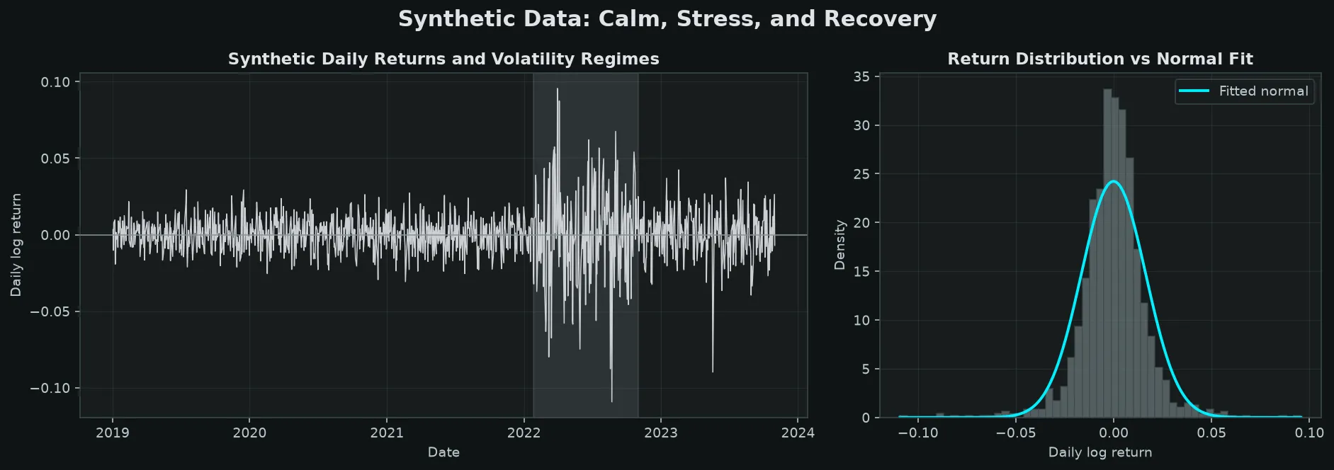
Rather than depend on a data feed, let us generate synthetic daily log returns with three volatility regimes — calm, stress, and recovery — to make the later analysis more interesting.
import numpy as np
import pandas as pd
from scipy import stats

rng = np.random.default_rng(42)

# 5 years of daily returns (1260 trading days)
n_days = 1260
dates = pd.bdate_range("2019-01-02", periods=n_days)

# Regime 1: calm  (days 0–800,   σ = 1.0% daily)
# Regime 2: stress (days 800–1000, σ = 3.0% daily — simulated crisis)
# Regime 3: recovery (days 1000–1260, σ = 1.5% daily)
mu = 0.00025  # ~6% annualized drift
vols = np.where(
    np.arange(n_days) < 800, 0.010,
    np.where(np.arange(n_days) < 1000, 0.030, 0.015)
)

# Add a fat-tail component: ~1% of days get a 3x shock
shocks = rng.standard_normal(n_days)
fat_tail = rng.choice([1.0, 3.0], size=n_days, p=[0.99, 0.01])
returns = pd.Series(
    mu + vols * shocks * fat_tail,
    index=dates,
    name="returns",
)

print(f"Total days:     {len(returns)}")
print(f"Mean daily ret: {returns.mean():.5f}")
print(f"Annualized vol: {returns.std() * np.sqrt(252):.2%}")
print(f"Skewness:       {returns.skew():.3f}")
print(f"Excess kurtosis:{returns.kurtosis():.3f}  (normal = 0)")
Total days: 1260
Mean daily ret: -0.00010
Annualized vol: 26.15%
Skewness: -0.325
Excess kurtosis: 6.174 (normal = 0)The sample's excess kurtosis of 6.174 indicates substantially heavier tails than a fitted normal distribution. Heavy tails and volatility clustering are also well-documented stylized facts of financial returns, although their magnitude depends on the asset, sample period, and sampling frequency.
Historical Simulation VaR
The simplest VaR approach requires no distributional assumptions.
Sort the last daily returns. VaR at confidence is the negative of the percentile:
At 99% confidence with a 250-day window, the 1st percentile lies around the third-worst observation. The exact value depends on the sample-quantile interpolation convention; pandas uses linear interpolation by default.
def historical_var(
    returns: pd.Series,
    window: int = 250,
    confidence: float = 0.99,
) -> pd.Series:
    """
    Rolling historical simulation VaR.
    Returns the positive loss that is exceeded with probability (1-confidence).
    """
    lagged = returns.shift(1)
    return (
        -lagged
        .rolling(window)
        .quantile(1 - confidence)
    ).rename(f"hist_var_{int(confidence*100)}")


def historical_es(
    returns: pd.Series,
    window: int = 250,
    confidence: float = 0.99,
) -> pd.Series:
    """Rolling historical Expected Shortfall (average loss beyond VaR)."""
    def tail_mean(x):
        threshold = np.quantile(x, 1 - confidence)
        tail = x[x <= threshold]
        return -tail.mean() if len(tail) > 0 else np.nan

    lagged = returns.shift(1)
    return (
        lagged
        .rolling(window)
        .apply(tail_mean, raw=True)
        .rename(f"hist_es_{int(confidence*100)}")
    )


hist_var_99 = historical_var(returns, window=250, confidence=0.99)
hist_es_99  = historical_es(returns, window=250, confidence=0.99)
Historical simulation has real advantages: it makes no parametric distributional assumption and preserves the skewness and tail behavior present in the selected window.
The cost: it looks backward. The window contains the past 250 observations and weights each one equally. If most of the past year was quiet, historical VaR can remain low as conditions deteriorate; it also updates in coarse jumps as observations enter and leave the tail.
Parametric VaR: Rolling Window
If we are willing to assume that daily returns are approximately normally distributed, we can estimate VaR analytically from the sample mean and standard deviation:
where is the standard normal quantile at level .
For 99% confidence, .
The sample statistics are estimated over a rolling window. This is the approach that underpinned much of 1990s and 2000s bank risk management.
from scipy.stats import norm


def parametric_var(
    returns: pd.Series,
    window: int = 250,
    confidence: float = 0.99,
) -> pd.Series:
    """Rolling parametric (normal) VaR."""
    z = norm.ppf(confidence)
    roll = returns.shift(1).rolling(window)
    mu_roll    = roll.mean()
    sigma_roll = roll.std(ddof=1)
    return (-(mu_roll - z * sigma_roll)).rename(f"param_var_{int(confidence*100)}")


def parametric_es(
    returns: pd.Series,
    window: int = 250,
    confidence: float = 0.99,
) -> pd.Series:
    """Rolling parametric Expected Shortfall under normality."""
    z = norm.ppf(confidence)
    roll = returns.shift(1).rolling(window)
    mu_roll    = roll.mean()
    sigma_roll = roll.std(ddof=1)
    # ES (positive loss) = -mu + sigma * phi(z_alpha) / (1 - alpha)
    es = -mu_roll + sigma_roll * norm.pdf(z) / (1 - confidence)
    return es.rename(f"param_es_{int(confidence*100)}")


param_var_99 = parametric_var(returns, window=250, confidence=0.99)
param_es_99  = parametric_es(returns, window=250, confidence=0.99)
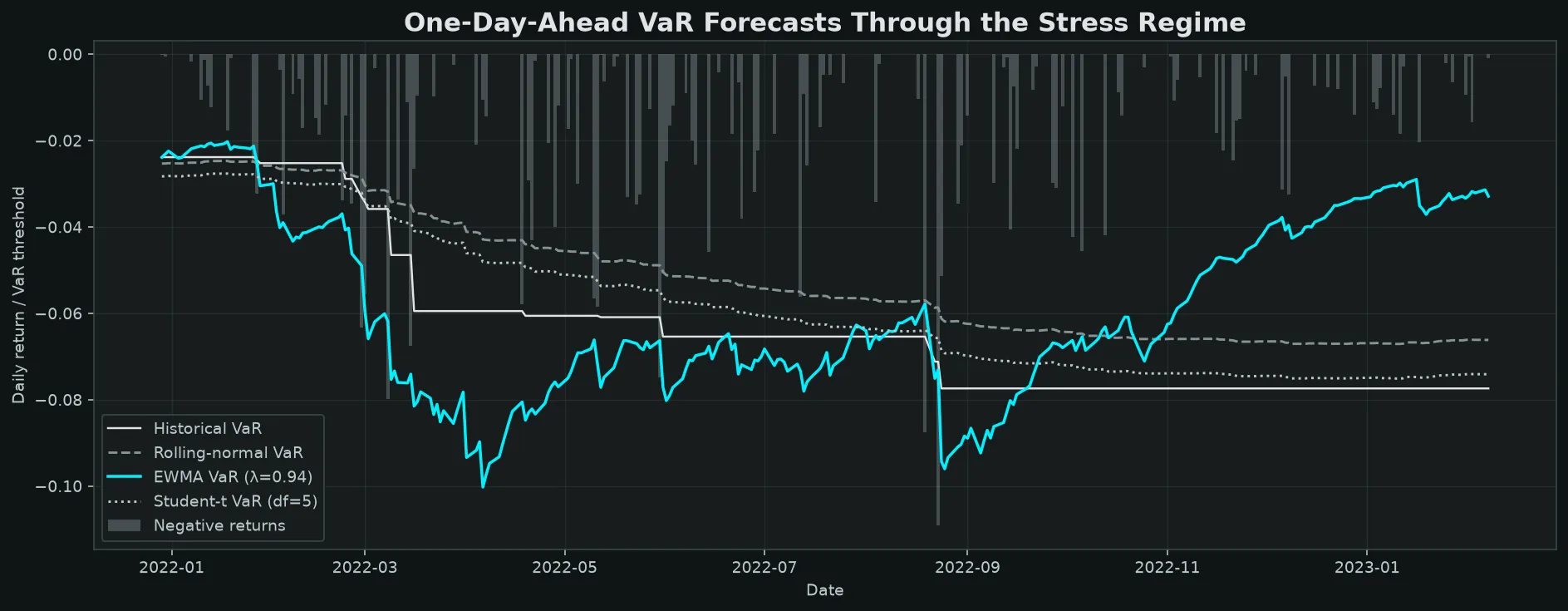
The rolling window parametric model is transparent and fast. Its failure mode is the same as the historical approach: a long window reacts slowly to volatility regime changes.
If the market was quiet for 200 of the past 250 days and then spiked, the parametric VaR still reflects mostly the quiet period. The signal arrives with a lag proportional to the window length.
EWMA VaR: The RiskMetrics Approach
The RiskMetrics innovation was to replace the uniform rolling window with exponentially decreasing weights. Recent returns matter more than old ones. Yesterday's return gets weight . The day before: . Two days ago: . And so on.
The EWMA variance recursion is:
This recursion is computationally trivial — update one number per day. The key parameter is , called the decay factor.
J.P. Morgan's RiskMetrics methodology specified for its daily dataset. The technical document describes choosing a single decay factor across hundreds of series using the root-mean-squared error of one-step-ahead variance forecasts.
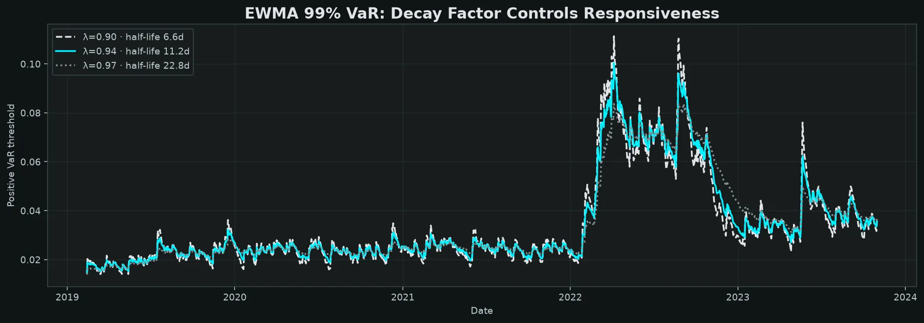
The decay factor has an intuitive interpretation: the half-life of information.
For : half-life trading days. After eleven days, the weight on a squared return in the variance estimate has halved. After 22 days, it has halved again. The memory decays geometrically.
Compare with a 250-day rolling window: a return from 249 days ago carries exactly the same weight as yesterday's return, then drops to zero on day 251. That cliff edge is both arbitrary and slow.
def ewma_var(
    returns: pd.Series,
    lam: float = 0.94,
    confidence: float = 0.99,
    min_periods: int = 30,
) -> pd.Series:
    """
    EWMA parametric VaR (RiskMetrics approach).
    Assumes zero mean (standard for daily VaR).
    """
    z = norm.ppf(confidence)

    # EWMA variance: σ²_t = λ σ²_{t-1} + (1-λ) r²_{t-1}
    squared = returns.shift(1) ** 2
    ewma_var_series = squared.ewm(
        alpha=1 - lam,
        min_periods=min_periods,
        adjust=False,
    ).mean()
    ewma_sigma = np.sqrt(ewma_var_series)

    return (z * ewma_sigma).rename(f"ewma_var_{int(confidence*100)}_lam{int(lam*100)}")


def ewma_es(
    returns: pd.Series,
    lam: float = 0.94,
    confidence: float = 0.99,
    min_periods: int = 30,
) -> pd.Series:
    """EWMA Expected Shortfall."""
    z = norm.ppf(confidence)
    squared = returns.shift(1) ** 2
    ewma_var_s = squared.ewm(
        alpha=1 - lam,
        min_periods=min_periods,
        adjust=False,
    ).mean()
    ewma_sigma = np.sqrt(ewma_var_s)
    es = ewma_sigma * norm.pdf(z) / (1 - confidence)
    return es.rename(f"ewma_es_{int(confidence*100)}_lam{int(lam*100)}")


ewma_var_94 = ewma_var(returns, lam=0.94, confidence=0.99)
ewma_es_94  = ewma_es(returns, lam=0.94, confidence=0.99)
Two details matter here. First, shift(1) makes the value dated a genuine forecast: it uses returns only through . Without the shift, a same-day loss would inflate its own risk threshold before the breach test, creating look-ahead bias. Second, pandas' smoothing parameter is ; this is unrelated to the VaR confidence level, so the code spells it out as alpha=1 - lam.
Comparing Decay Factors
A higher makes the model more sluggish — it forgets recent events slowly. A lower makes it react faster but noisier.
decay_factors = [0.90, 0.94, 0.97]
ewma_vars = {lam: ewma_var(returns, lam=lam, confidence=0.99) for lam in decay_factors}

half_lives = {lam: np.log(0.5) / np.log(lam) for lam in decay_factors}
print("Decay factor  Half-life (trading days)")
print("-" * 42)
for lam in decay_factors:
    print(f"  λ = {lam:.2f}      {half_lives[lam]:.1f} days")
Decay factor Half-life (trading days)
------------------------------------------
λ = 0.90 6.6 days
λ = 0.94 11.2 days
λ = 0.97 22.8 daysThe original RiskMetrics calibration used for its daily dataset and for its monthly dataset. Treat these as historical reference values, not universal constants: the appropriate decay depends on the series and forecast objective.
Scaling to Multi-Day Horizons
The legacy Basel internal-models framework used a 10-day, 99% VaR for market-risk capital. The current FRTB internal-models approach uses Expected Shortfall with liquidity-horizon adjustments instead. Under the strong assumption that daily returns are independent and identically distributed with finite variance, a volatility-based one-day VaR can be scaled by the square root of time:
def scale_var_to_horizon(var_1day: pd.Series, horizon_days: int = 10) -> pd.Series:
    """Scale 1-day VaR to a multi-day horizon using the square-root-of-time rule."""
    return (var_1day * np.sqrt(horizon_days)).rename(
        f"{var_1day.name}_scaled_{horizon_days}d"
    )

var_10day = scale_var_to_horizon(ewma_var_94, horizon_days=10)
var_1day_final = ewma_var_94.dropna().iloc[-1]
var_10day_final = var_10day.dropna().iloc[-1]
print(f"1-day EWMA VaR (99%): {var_1day_final:.4f}  (~{100 * var_1day_final:.2f}% of portfolio)")
print(f"10-day EWMA VaR (99%): {var_10day_final:.4f}  (~{100 * var_10day_final:.2f}% of portfolio)")
print(f"Ratio: {var_10day_final / var_1day_final:.4f}  (√10 = {np.sqrt(10):.4f})")
1-day EWMA VaR (99%): 0.0357 (~3.57% of portfolio)
10-day EWMA VaR (99%): 0.1129 (~11.29% of portfolio)
Ratio: 3.1623 (√10 = 3.1623)The square-root-of-time rule is a convenient model result, not a law. Serial dependence, changing conditional volatility, nonlinear positions, and compounding can all invalidate it. During a volatility transition it may understate or overstate multi-day risk, depending on how the one-day estimate relates to the volatility expected over the horizon.
Breach Testing: Does the Model Work?
A VaR model that cannot be checked is not a model — it is a belief.
Backtesting — also called breach testing or exception analysis — compares the VaR estimates against realized returns to verify that the model performs as advertised.
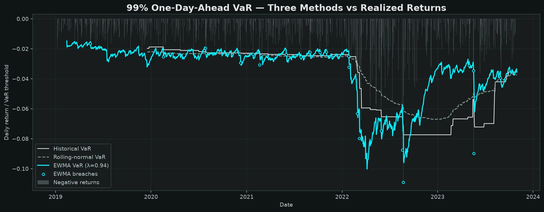
At 99% confidence, we expect the realized loss to exceed the VaR estimate on approximately 1% of days. Over 250 trading days, that means roughly 2.5 breaches per year.
- Too few breaches suggest that the model may be too conservative, although a small sample can also produce few exceptions by chance.
- Too many breaches suggest that the model is too optimistic — the dangerous direction.
def backtest_var(
    returns: pd.Series,
    var_series: pd.Series,
    confidence: float = 0.99,
) -> dict:
    """
    Backtest a VaR series against realized returns.
    Returns breach count, breach rate, expected rate,
    and Kupiec POF test statistic and p-value.
    """
    aligned = pd.DataFrame({"ret": returns, "var": var_series}).dropna()
    # A breach occurs when the loss (negative return) exceeds VaR
    aligned["breach"] = aligned["ret"] < -aligned["var"]

    T = len(aligned)
    V = aligned["breach"].sum()
    p = 1 - confidence           # expected breach probability
    p_hat = V / T                # observed breach rate

    # Kupiec Proportion of Failures (POF) test
    # LR = -2 ln[L(p) / L(p_hat)]
    # Under H0: breach rate = p, LR ~ chi-squared(1)
    ll_null = V * np.log(p) + (T - V) * np.log(1 - p)
    # At p_hat = 0 or 1, use the continuous limit 0 * log(0) = 0.
    ll_alt = 0.0
    if V > 0:
        ll_alt += V * np.log(p_hat)
    if V < T:
        ll_alt += (T - V) * np.log(1 - p_hat)

    lr_stat = -2 * (ll_null - ll_alt)
    kupiec_pval = stats.chi2.sf(lr_stat, df=1)

    return {
        "total_days":     T,
        "breaches":       int(V),
        "expected":       round(p * T, 1),
        "breach_rate":    round(p_hat * 100, 2),
        "expected_rate":  round(p * 100, 2),
        "kupiec_lr":      round(lr_stat, 3),
        "kupiec_pval":    round(kupiec_pval, 4),
    }
Let us run the backtest on all three VaR methods and print the results:
methods = {
    "Historical (250d)":  hist_var_99,
    "Parametric (250d)":  param_var_99,
    "EWMA (λ=0.94)":      ewma_var_94,
}

print(f"{'Method':<22} {'Days':>5} {'Breach':>7} {'Exp':>6} {'Rate%':>7} {'Exp%':>6} {'Kupiec p':>10}")
print("-" * 72)
for name, var_s in methods.items():
    r = backtest_var(returns, var_s, confidence=0.99)
    print(
        f"{name:<22} {r['total_days']:>5} {r['breaches']:>7} "
        f"{r['expected']:>6} {r['breach_rate']:>6.2f}% {r['expected_rate']:>5.2f}% "
        f"{str(r['kupiec_pval']):>10}"
    )
Method Days Breach Exp Rate% Exp% Kupiec p
------------------------------------------------------------------------
Historical (250d) 1010 23 10.1 2.28% 1.00% 0.0005
Parametric (250d) 1010 23 10.1 2.28% 1.00% 0.0005
EWMA (λ=0.94) 1230 23 12.3 1.87% 1.00% 0.0062The Kupiec p-value tests unconditional coverage: whether the total breach rate is statistically consistent with the target. At a chosen 5% test size, a p-value below 0.05 rejects that null hypothesis. A p-value above 0.05 does not prove the model is correct; it only says this test did not find enough evidence to reject it.
In this run:
- Historical simulation: p = 0.0005 — clear rejection. The backward-looking 250-day window was slow to react to the stress regime.
- Parametric rolling: p = 0.0005 — clear rejection. It has the same slow window turnover and adds a conditional-normal assumption.
- EWMA: p = 0.0062 — rejection at the 5% level. It has a lower breach rate than the two rolling-window models because it adapts faster, but the normal EWMA specification still does not calibrate this regime-switching, heavy-tailed sample adequately.
A model that cannot pass its own backtest is not a model. The Kupiec test is the minimum credibility check.
Kupiec's test also ignores the order of exceptions. Nine isolated breaches and nine consecutive breaches produce the same statistic, even though clustering is a serious warning sign. A fuller validation adds an independence or conditional-coverage test, such as Christoffersen's, and reviews exception severity as well as frequency.
The Basel Traffic Lights
Regulators formalized VaR backtesting in the 1996 Market Risk Amendment to the Basel Accord (later carried into Basel II). In the legacy framework, exceptions from one-day 99% VaR forecasts over the latest 250 trading days map to a traffic light:
| Breaches | Zone | Capital add-on (plus factor) |
|---|---|---|
| 0–4 | Green | 0 (baseline multiplier = 3×) |
| 5–9 | Yellow | 0.40–0.85 (multiplier 3.4×–3.85×) |
| 10+ | Red | 1.00 (multiplier 4×) |
In the yellow zone, the plus factor rises stepwise: 0.40, 0.50, 0.65, 0.75, and 0.85 for five through nine exceptions. The red-zone plus factor is 1.00. This is a pedagogical reproduction of the legacy VaR traffic-light calculation; the current FRTB framework adds Expected Shortfall, desk-level model eligibility, and other tests.
def basel_traffic_light(breaches: int, observations: int = 250) -> str:
    """Return the legacy Basel zone for a 250-observation backtest."""
    if observations != 250:
        raise ValueError("The published Basel thresholds are calibrated to 250 observations.")
    if breaches < 0:
        raise ValueError("breaches must be non-negative")

    noun = "breach" if breaches == 1 else "breaches"
    if breaches <= 4:
        return f"🟢 GREEN  ({breaches} {noun})"
    elif breaches <= 9:
        return f"🟡 YELLOW ({breaches} {noun})"
    else:
        return f"🔴 RED    ({breaches} {noun} — capital add-on applied)"


# Use last 250 days of each series for Basel assessment
for name, var_s in methods.items():
    last_250_ret = returns.iloc[-250:]
    last_250_var = var_s.reindex(last_250_ret.index).dropna()
    aligned = pd.concat([last_250_ret, last_250_var], axis=1).dropna()
    breaches_250 = (aligned.iloc[:, 0] < -aligned.iloc[:, 1]).sum()
    print(f"{name:<22}: {basel_traffic_light(breaches_250)}")
Historical (250d) : 🟢 GREEN (1 breach)
Parametric (250d) : 🟢 GREEN (1 breach)
EWMA (λ=0.94) : 🟢 GREEN (4 breaches)The final 250 observations all belong to the recovery regime; none comes from the simulated stress block. All three methods are therefore green in this particular window. That does not contradict the full-sample Kupiec results: the two diagnostics use different samples and answer different questions.
The Fat Tail Problem
Now comes the harder conversation.
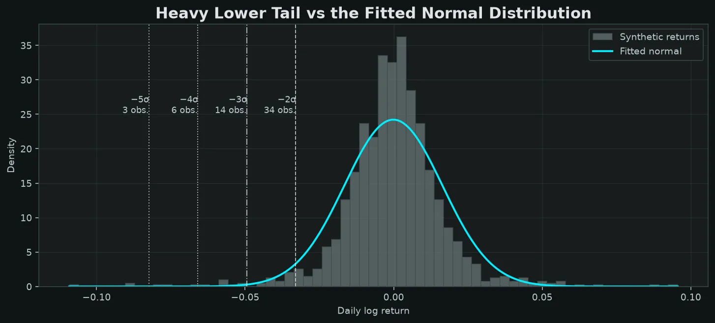
The two parametric models above assume conditionally normal daily returns. Historical simulation does not impose that distribution — one of its core advantages. Our synthetic data was explicitly constructed as a scale mixture, so its unconditional distribution has heavier tails than a normal distribution.
Excess kurtosis is one summary of tail weight. A normal distribution has excess kurtosis of zero, while empirical financial returns often show positive excess kurtosis. The estimate is highly sample-dependent and sensitive to extreme observations, so it should not be treated as a complete tail model.
What does this mean for VaR?
Under a standard normal distribution, a one-sided move below has probability — about once in 31,574 independent observations. Empirical return series often produce extreme moves more frequently than that Gaussian benchmark.
def compare_tail_probabilities():
    """Compare normal vs empirical tail probabilities."""
    sigma = returns.std()

    sigmas = [2.0, 3.0, 4.0, 5.0]
    print(f"{'Sigma level':>12} {'Normal prob':>14} {'Normal freq':>18} {'Empirical count':>16}")
    print("-" * 66)
    for s in sigmas:
        threshold = -s * sigma
        normal_prob = norm.cdf(threshold / sigma)
        normal_freq = f"once in {int(1/normal_prob):,} days"
        empirical_count = (returns < threshold).sum()
        print(
            f"{s:>10.0f}σ  {normal_prob:>12.2e}   {normal_freq:>18}   "
            f"{empirical_count:>8} actual days"
        )


compare_tail_probabilities()
Sigma level Normal prob Normal freq Empirical count
------------------------------------------------------------------
2σ 2.28e-02 once in 43 days 34 actual days
3σ 1.35e-03 once in 740 days 14 actual days
4σ 3.17e-05 once in 31,574 days 6 actual days
5σ 2.87e-07 once in 3,488,555 days 3 actual daysThe threshold, which a fitted Gaussian model assigns a probability of roughly one in 31,574, occurred six times in this 1,260-observation synthetic sample. The threshold occurred three times.
That result is a designed feature of this simulation, not empirical evidence: the 1% three-times-volatility mixture deliberately creates heavy tails. It illustrates a behavior also observed in many financial return series.
When the modeled lower tail is thinner than the true conditional tail, normal VaR will understate the relevant quantile. Breaches can then happen too often, and VaR still says nothing about their average severity.
Expected Shortfall: VaR's Better Sibling
VaR answers one question: how often do we lose more than ?
It says nothing about what happens when we do lose more than .
Expected Shortfall (ES) — also called Conditional VaR or CVaR in many continuous-distribution settings — fills that gap. For a continuous loss distribution, ES is the expected loss given that the loss exceeds VaR:
Under a normal distribution, the relationship is:
where and describe returns, losses are defined as negative returns, and is the standard normal PDF.
For a continuous loss distribution, ES is at least as large as VaR at the same confidence level. With zero-mean normal returns at 99%: .
But ES has a more fundamental advantage: under the standard quantile-averaging definition, it is a coherent risk measure. Specifically, it is subadditive — the ES of a portfolio is no greater than the sum of the ES of its positions. VaR does not have this property in general.
The Basel Committee's FRTB standard shifted the internal-models approach from VaR to Expected Shortfall under stress; the revised final standard was published in 2019. It uses 97.5% ES with liquidity horizons. For zero-mean normal returns, 97.5% ES and 99% VaR happen to be numerically close, but FRTB capital cannot be compared by confidence-level conversion alone because the framework also changed stress calibration, liquidity treatment, modellability, and aggregation.
# Compare VaR vs ES at the same confidence level
def full_comparison_table(returns, window=250, lam=0.94, confidence=0.99):
    h_var = historical_var(returns, window, confidence)
    h_es  = historical_es(returns, window, confidence)
    p_var = parametric_var(returns, window, confidence)
    p_es  = parametric_es(returns, window, confidence)
    e_var = ewma_var(returns, lam, confidence)
    e_es  = ewma_es(returns, lam, confidence)

    # Use last valid estimates
    last = lambda s: s.dropna().iloc[-1]

    print(f"\n99% VaR and Expected Shortfall — final estimate")
    print(f"{'Method':<22} {'VaR':>10} {'ES':>10} {'ES/VaR':>10}")
    print("-" * 56)
    for name, var_s, es_s in [
        ("Historical",     h_var, h_es),
        ("Parametric",     p_var, p_es),
        ("EWMA (λ=0.94)",  e_var, e_es),
    ]:
        v, e = last(var_s), last(es_s)
        print(f"{name:<22} {v:>9.4f}  {e:>9.4f}  {e/v:>9.2f}×")


full_comparison_table(returns)
99% VaR and Expected Shortfall — final estimate
Method VaR ES ES/VaR
--------------------------------------------------------
Historical 0.0355 0.0553 1.56×
Parametric 0.0376 0.0430 1.14×
EWMA (λ=0.94) 0.0357 0.0409 1.15×In this final synthetic-data forecast, ES is 14–56% larger than VaR depending on the method. The larger historical ratio reflects the few observations in that window beyond its interpolated VaR threshold; with only 250 observations at 99%, historical ES is based on a very small empirical tail and is correspondingly noisy.
Putting It Together: A Rolling Risk Dashboard
A useful risk dashboard reports VaR and ES from multiple methods, flags breaches, and tracks the rolling breach rate.
def rolling_breach_rate(
    returns: pd.Series,
    var_series: pd.Series,
    window: int = 60,
) -> pd.Series:
    """Rolling breach rate over a trailing window."""
    aligned = pd.DataFrame({"ret": returns, "var": var_series}).dropna()
    aligned["breach"] = (aligned["ret"] < -aligned["var"]).astype(float)
    return aligned["breach"].rolling(window).mean() * 100  # as percentage


# Dashboard summary
aligned = pd.DataFrame({
    "returns":   returns,
    "hist_var":  hist_var_99,
    "param_var": param_var_99,
    "ewma_var":  ewma_var_94,
    "hist_es":   hist_es_99,
    "ewma_es":   ewma_es_94,
}).dropna()

# Final 20 days snapshot
snapshot = aligned.tail(20).copy()
snapshot["ewma_breach"] = snapshot["returns"] < -snapshot["ewma_var"]

print(f"\nFinal 20 days — EWMA VaR vs realized returns")
print(f"{'Date':<12} {'Return':>9} {'EWMA VaR':>10} {'EWMA ES':>9} {'Breach':>8}")
print("-" * 54)
for date, row in snapshot.iterrows():
    breach_flag = "⚠️  BREACH" if row["ewma_breach"] else ""
    print(
        f"{str(date.date()):<12} "
        f"{row['returns']:>+8.4f}  "
        f"{row['ewma_var']:>9.4f}  "
        f"{row['ewma_es']:>8.4f}  "
        f"{breach_flag}"
    )
The dashboard pattern is the same one that fills trading floor risk screens daily: estimate a threshold, compare against reality, flag exceedances.
The difference between a professional risk system and a basic model is largely in the breach investigation. A rising exception rate can reflect misspecified dynamics, a regime change, data or P&L problems, or risks the model omits. Recalibration, new limits, hedging, or position reduction may follow, but the breach count alone does not prescribe the response.
The Failure Modes — What 2008 Showed
The financial crisis of 2008 is the canonical case study for VaR failure. But it is worth noting that the warning signs appeared a decade earlier.
In 1998, Long-Term Capital Management — a highly leveraged hedge fund known for convergence and relative-value trades — suffered losses severe enough to prompt a private-sector recapitalization coordinated by the Federal Reserve Bank of New York. The U.S. President's Working Group later documented the episode in its report on hedge funds, leverage, and LTCM. The failure was broader than a single VaR calculation: leverage, crowded positions, liquidity, and correlations all interacted under stress.
The 2007–09 crisis exposed similar weaknesses across a much larger financial system. Low pre-crisis volatility could make backward-looking measures look reassuring while leverage and illiquidity were building. In April 2008, the BIS noted that widely used VaR indicators had underestimated the rise in underlying position-taking during the low-volatility period.
There are several overlapping reasons:
1. Volatility clustering. Financial return volatility is not constant. Calm periods cluster with calm periods; volatile periods cluster with volatile periods. A model that assumes constant volatility or uses a slow-moving window will be badly miscalibrated at regime changes.
2. Correlation instability. Dependencies between assets can strengthen or change sign under stress. A portfolio diversified under ordinary-period estimates can become much more concentrated, causing a model calibrated to normal-period relationships to understate joint tail risk.
3. Liquidity gap. A short-horizon VaR built from mark-to-market P&L may not capture the time, market impact, or bid-ask cost required to unwind a large position. Under stress, those liquidation costs can dominate the modeled price move.
4. Tail misspecification. Financial returns often have heavier tails than a conditional normal model. The problem becomes multivariate: marginal tails and the dependence structure both matter, and ordinary-period covariance alone does not describe joint extremes.
The lesson is not that VaR is useless. It is that VaR is a starting point, not a destination.
VaR tells you how your portfolio behaves on a normal bad day. Risk management is about surviving the abnormal ones.
A mature risk framework uses VaR as one signal among many: stress tests, scenario analysis, reverse stress testing (what scenario would cause insolvency?), liquidity horizon adjustments, and — above all — the judgment to recognize when the model's assumptions no longer hold.
A Student's t VaR: Accounting for Fat Tails
One direct improvement is to replace the normal distribution with the Student's t distribution, which has heavier tails parametrized by its degrees of freedom .
For small , the tails are very heavy (resembling actual financial returns). As , the t distribution approaches the normal.
from scipy.stats import t as t_dist


def student_t_var(
    returns: pd.Series,
    window: int = 250,
    confidence: float = 0.99,
    df: int = 5,
) -> pd.Series:
    """
    Rolling parametric VaR using Student's t distribution.
    df: degrees of freedom (lower = fatter tails; must be greater than 2).
    """
    if df <= 2:
        raise ValueError("df must exceed 2 for a finite variance")

    # Scale factor: t distribution with df dof has variance df/(df-2)
    # We want the same empirical sigma, so scale the quantile
    scale_factor = np.sqrt(df / (df - 2))
    t_quantile = t_dist.ppf(confidence, df=df)
    # Effective z-equivalent = t_quantile / scale_factor
    effective_z = t_quantile / scale_factor

    roll = returns.shift(1).rolling(window)
    mu_roll = roll.mean()
    sigma_roll = roll.std(ddof=1)
    return (-mu_roll + effective_z * sigma_roll).rename(
        f"t_var_{df}df_{int(confidence*100)}"
    )


t_var_5df = student_t_var(returns, window=250, confidence=0.99, df=5)
result_t = backtest_var(returns, t_var_5df, confidence=0.99)

print(f"\nStudent-t VaR (df=5) backtest:")
print(f"  Breaches: {result_t['breaches']} (expected: {result_t['expected']})")
print(f"  Breach rate: {result_t['breach_rate']}% (target: {result_t['expected_rate']}%)")
print(f"  Kupiec p-value: {result_t['kupiec_pval']}")

result_norm = backtest_var(returns, param_var_99, confidence=0.99)
print(f"\nNormal VaR backtest for comparison:")
print(f"  Breaches: {result_norm['breaches']} (expected: {result_norm['expected']})")
print(f"  Kupiec p-value: {result_norm['kupiec_pval']}")
Student-t VaR (df=5) backtest:
Breaches: 18 (expected: 10.1)
Breach rate: 1.78% (target: 1.0%)
Kupiec p-value: 0.0244
Normal VaR backtest for comparison:
Breaches: 23 (expected: 10.1)
Kupiec p-value: 0.0005Both rolling models are rejected on unconditional coverage in this sample. The Student-t assumption reduces breaches from 23 to 18, but it does not eliminate the issue; improving the conditional tail shape does not make a 250-day volatility window adapt faster to a regime change.
Here, is an illustrative assumption, not an estimated parameter. In production, degrees of freedom and any location/scale dynamics should be estimated and validated out of sample; choosing a heavier-tailed marginal distribution does not by itself solve time-varying volatility.
The Takeaway
Value at Risk is the industry's shared language for daily market risk.
It is also a measure that requires constant skepticism.
Three things to remember:
1. VaR is a quantile, not a worst case. It tells you how often you lose more than , not how much you lose when you do. Expected Shortfall completes the picture.
2. Dynamics and tails are separate modeling problems. In this simulation, EWMA handles the volatility transition better while Student-t changes the conditional tail shape. Neither approach dominates universally; both assumptions must be validated.
3. Backtest the forecast you could actually have made. Shift every estimate so date uses information only through . Kupiec checks exception frequency; independence, severity, stress testing, and model governance complete the picture.
The next post extends this from single-position VaR to portfolio risk: how volatility is estimated, why constant-vol models fail, and what realized volatility and volatility clustering actually look like in data.
That is Volatility Is the Signal: From Black-Scholes Assumption to Market Reality.
Previous Posts in This Thread
- American Options and the Longstaff-Schwartz Algorithm — optimal stopping, backward induction, and LSM pricing.
- Monte Carlo Option Pricing: When Closed Forms Stop Helping — pricing path-dependent exotics with simulation.
- Black-Scholes Without the Magic — the PDE derivation and where closed forms come from.
- Geometric Brownian Motion in Python — GBM paths and log-return distributions.
- From Itô to Black-Scholes — the road from stochastic calculus to the pricing formula.
References
- J.P. Morgan, RiskMetrics — Technical Document, 4th Edition, 1996. The canonical EWMA specification used here.
- Philippe Jorion, Value at Risk: The New Benchmark for Managing Financial Risk, 3rd Edition, McGraw-Hill, 2006.
- Basel Committee on Banking Supervision, Amendment to the Capital Accord to Incorporate Market Risks, January 1996.
- Basel Committee on Banking Supervision, Minimum Capital Requirements for Market Risk, January 2019.
- Paul H. Kupiec, "Techniques for Verifying the Accuracy of Risk Measurement Models", Journal of Derivatives, 1995.
- Peter F. Christoffersen, "Evaluating Interval Forecasts", International Economic Review, 1998.
- Philippe Artzner, Freddy Delbaen, Jean-Marc Eber, and David Heath, "Coherent Measures of Risk", Mathematical Finance, 1999.
- Rama Cont, "Empirical Properties of Asset Returns: Stylized Facts and Statistical Issues", Quantitative Finance, 2001.
Get in Touch
Working on risk management infrastructure, regulatory capital models, or just exploring the CQF curriculum?
Connect with me:
- 📧 Email: [email protected]
- 🐦 Twitter/X: @TheDataGuyPro
- 💼 LinkedIn: Muhammad Afzaal
- 💻 GitHub: @mafzaal
- 🎥 YouTube: @TheDataGuyPro
- 🎧 Podcast: TheDataGuy Show
Whether you're building a risk system, studying for the CQF, or just trying to understand what your bank's 10-K means when it reports "99% 1-day VaR of $X billion," I'd love to hear from you!