
TabFM: Google's Zero-Shot Tabular Foundation Model for SPY Volatility
Every quant notebook eventually runs into the same repetitive loop: engineer features, train XGBoost, tune the window, tune the objective, tune the threshold, then start over when the target changes from returns to volatility.
That loop is not the model. It is the operating cost around the model.
Google Research's TabFM asks a sharp question: what if tabular prediction did not require a new training job for every dataset? What if a pretrained model could read the training rows, labels, and test rows as context, then produce classification or regression predictions in one forward pass?
That is the promise behind TabFM, Google's zero-shot foundation model for tabular data. It is also exactly the kind of claim worth testing on financial data, where the distributions are heavy-tailed, autocorrelated, regime-sensitive, and very good at humiliating generic machine learning claims.
This post breaks down the research and then turns it into a concrete experiment: forecasting next-period SPY realized volatility with a leakage-controlled tabular setup.
This continues our exploration of foundation models for structured data—previously, we looked at sequence-based event transformers in From Wall Street to ERP: Why Transformer Embeddings Are Eating Enterprise Transaction Systems, and here we test Google's zero-shot in-context learning model.
Contents
The Core Idea
TabFM treats a tabular dataset as an in-context learning problem.
In a normal supervised workflow, the dataset updates model parameters:
model.fit(X_train, y_train)
prediction = model.predict(X_test)
With TabFM, the pretrained model is already fixed. The rows and columns become the prompt. The model receives:
- feature columns for training rows
- labels for training rows
- feature columns for target rows
- missing labels for target rows
Then it predicts the missing labels in a single forward pass.
That sounds small until you think about how tabular ML is actually practiced. The expensive part is rarely the final .fit() call. The expensive part is the human loop around it: feature shaping, split design, hyperparameter search, calibration, ensembling, and retraining for every new task.
TabFM is an attempt to compress that loop into a pretrained prior over table structure.
How TabFM Reads a Table
Tables are not natural transformer inputs. Text is a one-dimensional sequence. A table is a two-dimensional object where both rows and columns matter.
TabFM uses an architecture designed for that geometry:
| Stage | Purpose |
|---|---|
| Row and column attention | Learns relationships across examples and features instead of flattening the table into one long string. |
| Row compression | Turns each row's cross-attended representation into a dense vector so the later transformer can scale. |
| ICL transformer | Performs in-context prediction over compressed row embeddings. |
| Classification or regression head | Produces task-specific outputs without updating the foundation model weights. |
The research note in this repo captured the practical version of the architecture:
embed_dim: 256
column blocks: 3
row blocks: 3
ICL transformer blocks: 24
ICL attention heads: 8
max classes: 10
The important design choice is not any single number. It is the separation of concerns: learn feature interactions, compress rows, then reason over row-level context.
That is the tabular equivalent of asking a language model to read a few examples before answering a new question.
The Synthetic Data Bet
The most interesting part of TabFM is not that it uses a transformer. It is that Google trained it on synthetic data.
Real enterprise tables are valuable, private, schema-specific, and legally awkward to pool at frontier-model scale. Google sidesteps that by generating hundreds of millions of synthetic tabular tasks from structural causal models.
The bet is subtle:
The values can be synthetic as long as the statistical structure teaches the model useful priors about how tabular features interact.
That could work very well for many business problems. Vendor payment delays, churn, fraud triage, loan default, and claims risk all have recurring table shapes: mixed numerical and categorical features, missingness, nonlinear interactions, and feature redundancy.
Markets are less forgiving. Equity volatility has regime shifts, volatility clustering, calendar effects, exogenous shocks, and tail behavior that simple synthetic causal generators may not capture. That does not make TabFM useless for finance, but it does change the test.
For market data, the question is not:
Does TabFM beat tuned XGBoost on a static leaderboard?
The better question is:
Does TabFM add useful, leakage-free signal under chronological validation, after simple volatility baselines already exist?
Benchmarks Are a Starting Point
Google reports TabFM against TabArena, a benchmark suite with classification and regression datasets scored through head-to-head Elo-style comparisons. The release materials describe strong results against tuned tree-based baselines such as XGBoost, LightGBM, Random Forest, and CatBoost.
That is impressive, but benchmark wins are not the same thing as production readiness.
For finance, I would want to know:
- whether train and test periods are separated chronologically
- whether the model sees any future-normalized features
- how it behaves during volatility regime shifts
- whether its errors are calibrated, not just low on average
- whether it beats trivial baselines like yesterday's realized volatility or EWMA
- whether the edge survives transaction-cost-aware downstream decisions
Volatility forecasting is a good first diagnostic because the target is measurable, economically meaningful, and hard enough to expose overfit models.
The License Boundary
The license matters here.
The GitHub code is useful for studying the architecture and running experiments. The pretrained weights on Hugging Face are distributed under Google's TabFM non-commercial license. The practical boundary is simple:
- fine for research, education, and evaluation
- not fine for production trading, commercial risk products, or revenue-generating services without a separate commercial license
That makes the right mental model:
TabFM is a research tool today, not a plug-and-play production quant dependency.
For a public SPY volatility notebook, that is acceptable. For a deployed signal pipeline, it is not enough.
A SPY Volatility Forecasting Test
The notebook frames the problem as supervised tabular regression:
Given only information available at the close of day , forecast the realized volatility over the next 21 trading days.
The target is forward realized volatility:
The features are deliberately boring:
| Feature group | Examples |
|---|---|
| Return memory | 1-day, 5-day, 21-day, and 63-day returns |
| Realized volatility | 5-day, 21-day, and 63-day annualized vol |
| Range features | intraday high-low range, close-open return |
| Volume pressure | volume z-score and volume trend |
| Volatility ratios | short volatility divided by medium volatility |
| Calendar state | month, day of week, month-end flag |
The notebook uses real SPY data when yfinance is available. If the environment has no network access, it falls back to a deterministic SPY-like synthetic OHLCV series so the feature pipeline, split logic, model wrapper, and plots still run.
That fallback is not there to fake market evidence. It is there to make the notebook executable in restricted environments.
For the run below, yfinance succeeded. The dataset covered 5,406 SPY daily bars from January 3, 2005 through June 30, 2026. After feature engineering and forward-target construction, the supervised frame had 5,341 rows.
The chronological split was:
| Split | Date range | Rows |
|---|---|---|
| Train | 2005-04-05 to 2019-01-16 | 3,471 |
| Validation | 2019-01-17 to 2022-03-22 | 801 |
| Test | 2022-03-23 to 2026-06-26 | 1,069 |
The target was not quiet. Across the engineered sample, 21-day forward realized volatility had a mean of 15.7%, median of 13.0%, and max of 93.7% annualized. In other words: the test is not just "can the model fit calm periods?"
The Exact Target Code
The target construction is the part I care about most, because this is where leakage usually slips in. The notebook builds the next-21-day target from future returns only after features have been computed from current and past data:
def forward_realized_vol(log_returns, horizon=21):
    future = pd.concat(
        [log_returns.shift(-i).rename(f"r_plus_{i}") for i in range(1, horizon + 1)],
        axis=1,
    )
    return future.std(axis=1, ddof=1) * np.sqrt(252)
Then the feature table adds rolling returns, rolling volatility, range-based features, volume pressure, and calendar state:
df["log_return_1d"] = np.log(df["Close"]).diff()
df["return_5d"] = np.log(df["Close"]).diff(5)
df["return_21d"] = np.log(df["Close"]).diff(21)
df["return_63d"] = np.log(df["Close"]).diff(63)

for window in [5, 10, 21, 63]:
    df[f"vol_{window}d"] = df["log_return_1d"].rolling(window).std() * np.sqrt(252)

df["ewma_vol_21d"] = df["log_return_1d"].ewm(span=21, adjust=False).std() * np.sqrt(252)
df["hl_range"] = np.log(df["High"] / df["Low"])
df["parkinson_vol_21d"] = np.sqrt(
    252.0 * (df["hl_range"] ** 2).rolling(21).mean() / (4.0 * np.log(2.0))
)
df["target_vol_21d"] = forward_realized_vol(df["log_return_1d"], horizon=21)
This is the minimal table I would hand to TabFM: mixed market-state columns, one scalar regression target, and no random split.
Leakage Controls
The most important part of the notebook is not the model call. It is the validation design.
The notebook uses:
- chronological train, validation, and test splits
- forward targets shifted so features at day never contain returns from day onward
- rolling features computed only from current and past observations
- simple baselines before any foundation model score is celebrated
- regression metrics reported on the final holdout period only
The baselines are intentionally hard to embarrass:
baseline_yesterday = test["vol_21d"]
baseline_ewma = test["ewma_vol_21d"]
If TabFM cannot clear those, the foundation-model story does not matter for this task.
The split code is intentionally boring:
def chronological_split(df, train_frac=0.65, val_frac=0.15):
    n = len(df)
    train_end = int(n * train_frac)
    val_end = int(n * (train_frac + val_frac))
    return (
        df.iloc[:train_end].copy(),
        df.iloc[train_end:val_end].copy(),
        df.iloc[val_end:].copy(),
    )
Running TabFM on CUDA
I installed the PyTorch backend from the official Google Research repository and used a CUDA-enabled PyTorch build on an NVIDIA GeForce RTX 5080 Laptop GPU:
pip install torch torchvision torchaudio --index-url https://download.pytorch.org/whl/cu128

git clone https://github.com/google-research/tabfm.git
cd tabfm
pip install ".[pytorch]"
TabFM's README is explicit about the order: install the right PyTorch build for your CUDA version first, then install tabfm[pytorch].
The regression model loads like a normal PyTorch module. For this volatility task, the important line is model_type="regression":
import torch
from tabfm import TabFMRegressor
from tabfm import tabfm_v1_0_0_pytorch as tabfm_v1_0_0

device = "cuda" if torch.cuda.is_available() else "cpu"
foundation_model = tabfm_v1_0_0.load(model_type="regression", device=device)

regressor = TabFMRegressor(
    model=foundation_model,
    n_estimators=1,
    norm_methods="none",
    feat_shuffle_method="none",
    batch_size=1,
    enable_nnls=False,
    random_state=42,
)

regressor.fit(train_val[feature_cols], train_val[target_col].to_numpy())
tabfm_pred = regressor.predict(test[feature_cols])
The .fit() call deserves a warning: this is not training the TabFM weights. It prepares the sklearn-style preprocessing and gives the model the train+validation rows as in-context examples. The foundation model remains frozen.
I ran three TabFM configurations:
| Configuration | Context rows | Test rows | GPU prediction time |
|---|---|---|---|
| TabFM 1x CUDA | 4,272 | 1,069 | 4.3 seconds |
| TabFM 4x CUDA | 4,272 | 1,069 | 18.0 seconds |
| TabFM 8x CUDA | 4,272 | 1,069 | 51.5 seconds |
The one-time model load took about 67.5 seconds after the Hugging Face snapshot was cached. That load time is not the same as per-run inference latency, but it matters if you are thinking about batch jobs.
Findings from the Full Comparison
Before judging TabFM, the notebook runs three classical volatility baselines plus a small supervised ridge model. The ridge model is not meant to be impressive. It is there to answer a practical question:
Does even a simple tabular learner extract incremental signal from the engineered market-state features?
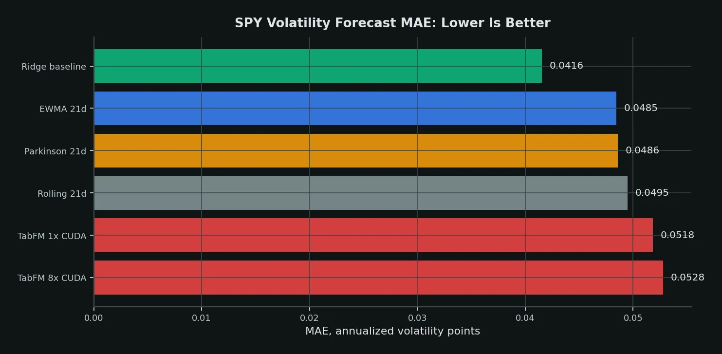
On the 2022-2026 test window, the answer was yes. TabFM, however, did not clear that hurdle:
| Model | MAE | RMSE | Pearson corr | Spearman corr |
|---|---|---|---|---|
| Ridge baseline | 0.0416 | 0.0654 | 0.568 | 0.619 |
| EWMA 21-day vol | 0.0485 | 0.0760 | 0.501 | 0.526 |
| Parkinson 21-day vol | 0.0486 | 0.0750 | 0.519 | 0.564 |
| Rolling 21-day vol | 0.0495 | 0.0786 | 0.484 | 0.518 |
| TabFM 1x CUDA | 0.0518 | 0.0830 | 0.386 | 0.410 |
| TabFM 4x CUDA | 0.0530 | 0.0870 | 0.366 | 0.404 |
| TabFM 8x CUDA | 0.0528 | 0.0855 | 0.374 | 0.405 |
That is the kind of result I want from this experiment, even though it is not the result a TabFM headline would want. A basic ridge model cut MAE by about 14% versus EWMA and about 16% versus rolling 21-day volatility. TabFM 1x was about 25% worse than ridge and about 7% worse than EWMA on MAE.
The metric comparison is the cleanest view:
The time-series chart shows why:
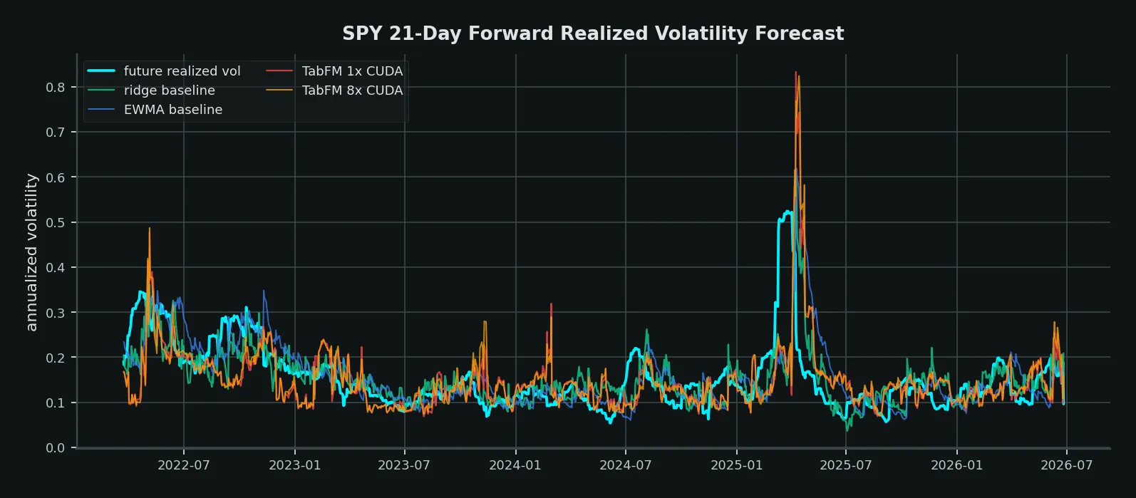
First, every model is late to the 2025 volatility shock. That is expected: the target is forward-looking and the features only know the past. A model that perfectly anticipates a shock from no information would be suspicious.
Second, TabFM tends to inject sharper prediction spikes than the ridge baseline. It sometimes reacts to market-state features in the right direction, but the amplitude is not calibrated for this volatility target.
The diagnostic chart makes the calibration issue clearer:
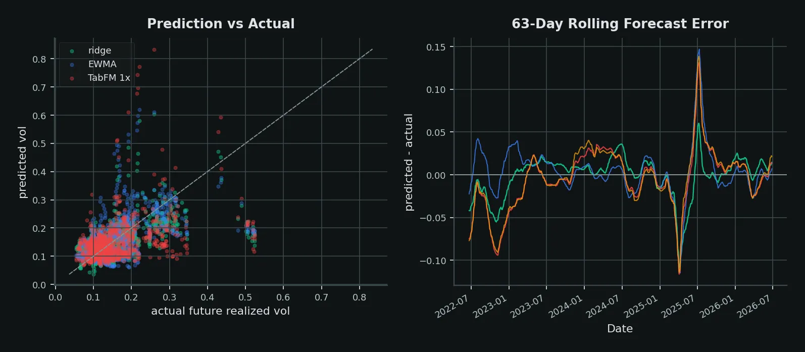
This is the first real hurdle for TabFM. It does not merely need to beat a naive rolling-vol number. It needs to beat a regularized tabular baseline that already learns something useful from lagged returns, range features, and volume pressure.
The Supervised Baseline Code
Here is the fallback ridge model from the notebook. It is deliberately implemented with NumPy so the comparison has one dependency-light supervised baseline:
def fit_ridge_numpy(X, y, alpha=1.0):
    X = np.asarray(X, dtype=float)
    y = np.asarray(y, dtype=float)
    X_design = np.column_stack([np.ones(len(X)), X])
    penalty = alpha * np.eye(X_design.shape[1])
    penalty[0, 0] = 0.0
    coef = np.linalg.solve(X_design.T @ X_design + penalty, X_design.T @ y)
    return coef


def predict_ridge_numpy(X, coef):
    X = np.asarray(X, dtype=float)
    X_design = np.column_stack([np.ones(len(X)), X])
    return np.clip(X_design @ coef, 0.0, None)
The validation loop chose the ridge penalty on the validation period, then refit on train plus validation before scoring the final test period:
alphas = np.logspace(-4, 4, 25)
val_rows = []

for alpha in alphas:
    coef = fit_ridge_numpy(X_train, y_train, alpha=alpha)
    pred_val = predict_ridge_numpy(X_val, coef)
    val_rows.append({
        "alpha": alpha,
        "MAE": mean_absolute_error(y_val, pred_val),
        "RMSE": root_mean_squared_error(y_val, pred_val),
    })

best_alpha = pd.DataFrame(val_rows).sort_values("MAE").iloc[0]["alpha"]
This is not the model I ultimately care about. It is the audit trail. If a larger model cannot clear this baseline, the experiment stops there.
What This Result Means
For SPY volatility, this run does not support replacing classical baselines with TabFM. The model executed correctly on GPU, but the forecasts were less accurate and less rank-correlated than the simple ridge baseline.
That does not make TabFM a failure. It narrows the claim:
- TabFM did run zero-shot on a real SPY volatility table with 4,272 context rows.
- GPU inference was practical: about 4.3 seconds for the single-member forecast after model load.
- The generic tabular prior did not transfer cleanly to this market-volatility target.
- A tiny task-specific ridge model won because it only had to learn a narrow volatility mapping from carefully chosen features.
The next test I would run is not "try a bigger ensemble and hope." It is more targeted:
- change the target to volatility regime classification instead of point regression
- test shorter context windows instead of the full 2005-2022 history
- add VIX, rates, credit spreads, and macro state rather than using SPY-only OHLCV
- ensemble TabFM with ridge/EWMA and test whether it contributes independent residual signal
If TabFM becomes useful here, I expect it to be as a feature generator or weak ensemble member, not as a standalone volatility forecaster.
The Practical Takeaway
TabFM is one of the most interesting tabular ML releases of 2026 because it attacks the real bottleneck: repeated, dataset-specific model building.
For enterprise data, the zero-shot path could be transformative. For finance, it deserves a colder evaluation. Market data is non-stationary, noisy, and adversarial in ways benchmark tables usually are not.
That is why the SPY notebook is framed as a test harness, not a victory lap. It produced a useful negative result: TabFM's zero-shot prior is not automatically better than a small, leakage-controlled model for market volatility.
Run TabFM against simple volatility baselines. Keep the split chronological. Check the regime behavior. Respect the non-commercial license. Then decide whether the foundation-model prior is adding signal or just adding novelty. In this first pass, it added novelty, not signal.
The Jupyter notebook for this post is available for download: tabfm-spy-volatility-forecast.ipynb.
But the important part is now in the article itself: the target, the split, the CUDA TabFM run, the baseline metrics, the charts, and the exact hurdle TabFM failed to clear.
References
- Google Research, Introducing TabFM: A zero-shot foundation model for tabular data
- Google Research, TabFM GitHub repository
- Hugging Face, google/tabfm-1.0.0-pytorch
- Hollmann et al., TabPFN: A Transformer That Solves Small Tabular Classification Problems in a Second
- Qu et al., TabICL: A Tabular Foundation Model for In-Context Learning on Large Data