Geometric Brownian Motion in Python: The First Model Every Quant Learns

Monday morning. A clean notebook. A blank chart.

You are not trying to predict the market yet. That comes later, and if you are honest, it will come with caveats, backtests, leakage checks, regime breaks, transaction costs, and a lot of humility.

For now, the first quant finance problem is smaller.

You need a model of a price path.

Not a perfect model. Not a trading strategy. Not a machine that turns historical candles into certainty. Just a first mathematical world where prices move randomly, returns compound, volatility matters, and risk can be simulated.

That first world is usually geometric Brownian motion.

In the previous bridge post, we followed the story from Itô's calculus to Black-Scholes-Merton. The key idea was that a random stock path could be transformed into a pricing equation for a derivative.

But that story depends on a simpler object underneath it:

$$d{S}_t=\mu S_{t}dt+\sigma S_{t}d{W}_t$$

That line is geometric Brownian motion, or GBM.

This post slows down and turns that line into something practical. We will connect the intuition, the math, and a small Python simulation. The goal is not to build a market forecast. The goal is to understand the baseline model that sits under a large part of modern quant finance.

This is educational research, not investment advice.

Contents

---

The First Mistake: Modeling Prices Instead of Returns

Imagine a stock trading at $10.

A one-dollar move is large. It is 10%.

Now imagine a stock trading at $1,000.

A one-dollar move is noise. It is 0.1%.

This is the first reason finance usually thinks in returns rather than raw price changes. A dollar is not the same unit of risk at every price level. A percentage move is closer to the language markets actually speak.

Bachelier's 1900 thesis treated speculation with Brownian-style price changes. That was a brilliant beginning. But arithmetic Brownian motion has a practical problem when used directly for stocks:

$$d{S}_t=\mu dt+\sigma d{W}_t$$

The noise does not care where the price is. The same absolute shock can hit a cheap stock and an expensive stock. Worse, the process can wander below zero.

That is not automatically wrong for every financial variable. Some rates and spreads can be negative. But for an ordinary equity price, negative values are a bad first model.

GBM changes the unit of motion.

Instead of making the absolute price change random, it makes the percentage change random:

$$\frac{d{S}_t}{S_t}=\mu dt+\sigma d{W}_t$$

or equivalently:

$$d{S}_t=\mu S_{t}dt+\sigma S_{t}d{W}_t$$

The drift term scales with price. The volatility term scales with price. If the price doubles, the same percentage volatility produces larger dollar swings.

That sounds simple, but it changes the whole geometry of the model.

Prices stay positive. Returns become the natural object. Logarithms enter the story.

---

The Model in Plain English

GBM has two forces.

The first is drift:

$$\mu S_{t}dt$$

Think of this as the smooth trend part. If there were no randomness, the price would grow or decay exponentially.

The second is noise:

$$\sigma S_{t}d{W}_t$$

This is the Brownian shock. The parameter $\sigma$ is volatility. It controls how wide the possible paths spread over time.

Put them together:

$$d{S}_t=\mu S_{t}dt+\sigma S_{t}d{W}_t$$

The story is:

• the asset has an expected percentage drift;
• shocks arrive continuously;
• shock size is proportional to the current price;
• the path remains positive;
• uncertainty compounds.

Random Services' mathematical notes define GBM in exactly this exponential Brownian-motion form and show that it satisfies the SDE above. That exponential form is what we will simulate in Python.

But before the code, there is one correction term worth respecting.

---

The Small Term That Changes the Story

If ordinary calculus were enough, you might guess that taking logs gives:

$$d\log (S_t)\approx \mu dt+\sigma d{W}_t$$

But ordinary calculus is not enough. Brownian motion has quadratic variation. Itô's lemma adds the correction:

$$d\log (S_t)=\left(\mu -\frac{1}{2}{\sigma }^2\right)dt+\sigma d{W}_t$$

That means the exact solution is:

$$S_t=S_0\exp \left(\left(\mu -\frac{1}{2}{\sigma }^2\right)t+\sigma W_t\right)$$

The expected price grows with $\mu$:

$$E[S_t]=S_0{e}^{\mu t}$$

But the expected log growth rate is lower:

$$E\left[\log (S_t/S_0)\right]=\left(\mu -\frac{1}{2}{\sigma }^2\right)t$$

That gap is not a technical footnote. It is the first practical finance lesson in the model.

Volatility does not merely create a cloud around the trend. It changes the growth rate experienced by a compounded path.

This is why quant finance is so careful about return definitions. Arithmetic returns, log returns, expected terminal price, median terminal price, and pathwise growth are related, but they are not the same thing.

GBM makes that difference visible early.

---

Simulating GBM in Python

There are two common ways to simulate this model.

One is to step through the SDE directly with an approximation method. That is useful later.

For this introduction, we can use the exact log-return step:

$$\log (S_{t+\Delta t}/S_t)=\left(\mu -\frac{1}{2}{\sigma }^2\right)\Delta t+\sigma \sqrt{\Delta t}Z$$

where $Z$ is a standard normal random variable.

Here is a minimal vectorized simulation:

import numpy as np


def simulate_gbm(
    s0: float,
    mu: float,
    sigma: float,
    years: float,
    steps_per_year: int,
    n_paths: int,
    seed: int = 7,
) -> np.ndarray:
    rng = np.random.default_rng(seed)
    n_steps = int(years * steps_per_year)
    dt = years / n_steps

    shocks = rng.standard_normal((n_paths, n_steps))
    log_returns = (
        (mu - 0.5 * sigma**2) * dt
        + sigma * np.sqrt(dt) * shocks
    )

    log_paths = np.cumsum(log_returns, axis=1)
    log_paths = np.concatenate(
        [np.zeros((n_paths, 1)), log_paths],
        axis=1,
    )

    return s0 * np.exp(log_paths)


paths = simulate_gbm(
    s0=100.0,
    mu=0.08,
    sigma=0.20,
    years=1.0,
    steps_per_year=252,
    n_paths=10_000,
)

This code is doing something specific:

• s0=100.0 starts every path at 100;
• mu=0.08 sets an 8% annual drift assumption;
• sigma=0.20 sets a 20% annual volatility assumption;
• steps_per_year=252 uses a trading-day grid;
• n_paths=10_000 creates a distribution of possible one-year outcomes.

Notice what it does not do.

It does not download market data. It does not fit parameters. It does not claim that tomorrow's market follows this process. It only asks:

If this simple model were true, what kind of paths would we see?

That question is already useful.

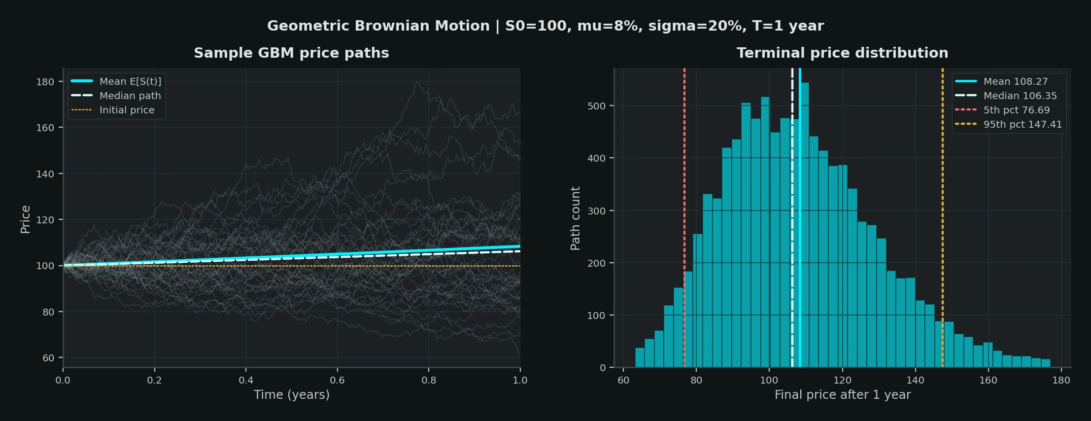
The image uses the same exact log-return simulation: $S_0=100$, $\mu =8\%$, $\sigma =20\%$, 252 trading steps, and a fixed seed. The muted lines are individual sample paths; the cyan line is the analytical mean $E[S_t]=S_0{e}^{\mu t}$. Notice how quickly the paths fan out even though every path starts from the same price and shares the same model assumptions.

---

What the Simulation Teaches

Once the paths exist, we can look at terminal outcomes:

terminal = paths[:, -1]
terminal_returns = terminal / paths[:, 0] - 1.0

summary = {
    "mean_terminal_price": np.mean(terminal),
    "median_terminal_price": np.median(terminal),
    "probability_of_loss": np.mean(terminal < paths[:, 0]),
    "five_percent_return_quantile": np.quantile(terminal_returns, 0.05),
    "ninety_five_percent_return_quantile": np.quantile(terminal_returns, 0.95),
}

The exact numbers will move with the seed and parameters, but the pattern matters more than the specific output.

The mean terminal price is pulled upward by the right tail. GBM produces a lognormal terminal distribution, so large positive outcomes can stretch the average.

The median terminal price is usually lower than the mean. That is the compounding story. One very strong path can lift the average, but the median path tells you where the middle outcome lands.

The probability of loss can be meaningful even when the drift is positive. A positive expected return does not mean most paths make money over a short horizon.

The lower quantile gives the first hint of risk measurement. Without using the full language of Value at Risk yet, we are already asking: what does a bad but not impossible outcome look like under this model?

That is the quant habit forming.

Define the model. Simulate the distribution. Measure the downside. Then ask whether the assumptions deserve trust.

---

The Parameters Are Not Equal

GBM has two headline parameters: $\mu$ and $\sigma$.

They look symmetric in the equation.

They are not symmetric in practice.

Volatility is noisy, but it is more observable than drift. You can estimate realized volatility from historical returns over a window and get something usable as a rough input. It will still change. It will cluster. It will break during stress. But it leaves a stronger statistical footprint.

Drift is much harder.

Expected return is a small signal buried under large noise. Over days and weeks, volatility dominates. Over months, uncertainty remains large. Even over years, the estimate can be unstable because regimes change and the sample is small relative to the noise.

This is one reason derivatives pricing under Black-Scholes-Merton is so striking. In the idealized hedge argument, the expected stock return $\mu$ drops out of the pricing equation. The option price depends on volatility, time, strike, spot, rates, and carry assumptions, not your private estimate of expected stock drift.

That does not make drift irrelevant for every problem. Portfolio construction, forecasting, allocation, and strategy research still care about expected returns.

But it explains why the first quant instinct is often:

be skeptical of drift, be disciplined about volatility.

---

Why GBM Survived Despite Being Wrong

GBM is wrong in obvious ways.

Volatility is not constant. Markets jump. Returns have fat tails. Liquidity changes. Correlations rise in stress. Trading is discrete. Transaction costs exist. The model has no earnings announcements, central-bank surprises, order books, forced liquidations, or changing regimes.

Robert Engle's ARCH work became important precisely because financial volatility changes over time. The Nobel Prize 2003 press release notes that turbulent periods with large fluctuations are followed by calmer periods with smaller fluctuations, and that constant-volatility methods were often used before better alternatives became available.

That sounds like a direct criticism of GBM.

It is.

But a flawed baseline can still be valuable.

GBM survived because it is analytically clean. It keeps prices positive. It gives lognormal terminal prices. It connects directly to Itô calculus. It makes Black-Scholes possible. It is easy to simulate. It gives a common reference point from which more realistic models can depart.

In practice, a baseline model earns its place when it helps you see the size and direction of its own mistakes.

GBM does that.

When implied volatility forms a smile, the market is telling you that constant volatility is not enough. When realized returns show fat tails, the data is telling you normal log shocks are too polite. When volatility clusters, the time series is telling you that a fixed $\sigma$ is too rigid.

The model is not the final answer.

It is the first coordinate system.

---

Where Machine Learning Enters

This is also where the bridge to machine learning becomes natural.

Machine learning should not enter the story as magic alpha dust sprinkled over price charts. That is the fastest way to fool yourself.

It enters because the clean model leaves estimation problems behind.

Instead of assuming one constant volatility, can we estimate volatility regimes?

Instead of treating every day as identically distributed, can we condition on macro variables, realized volatility, liquidity, trend, or cross-asset stress?

Instead of training on random splits that leak the future, can we use walk-forward validation?

Instead of optimizing a classification metric that never touches P&L, can we evaluate calibrated probabilities, drawdowns, turnover, transaction costs, and breach behavior?

The stochastic model gives us the nouns:

• return;
• volatility;
• diffusion;
• drift;
• log growth;
• tail risk;
• path;
• hedge;
• calibration.

Machine learning gives us another way to estimate relationships among those nouns from messy data.

That is the transition I want this series to make slowly. The goal is not to abandon the mathematics. The goal is to carry the mathematics into the research workflow.

---

The Takeaway

GBM is the first model every quant learns because it is small enough to hold in your head and large enough to teach the main lessons.

It teaches that prices should often be modeled through returns.

It teaches that log returns are not a cosmetic transformation.

It teaches that volatility changes growth accounting.

It teaches that a distribution of paths is more honest than a single forecast.

It teaches that model assumptions are not fine print; they are the boundary of the result.

And it prepares the next step.

Once we can simulate the stock path, we can place a payoff on top of it. Then the question changes from:

Where might the stock go?

to:

What is the fair price of a promise written on that uncertainty?

That is where Black-Scholes returns, this time without the magic.

---

References

• Random Services, Geometric Brownian Motion.
• Fischer Black and Myron Scholes, "The Pricing of Options and Corporate Liabilities", Journal of Political Economy, 1973.
• Robert C. Merton, "Theory of Rational Option Pricing", The Bell Journal of Economics and Management Science, 1973.
• Nobel Prize, The Prize in Economic Sciences 1997 - Press release, October 14, 1997.
• Nobel Prize, The Prize in Economic Sciences 2003 - Press release, October 8, 2003.
• Louis Bachelier, Theory of Speculation, 1900 thesis translation.