Black-Scholes Without the Magic: Turning Random Paths into a Pricing Equation

The Geometric Brownian Motion in Python: Your First Quant Model post ended with a random stock path.

Not a prediction. Not a signal. Not a model of every strange thing markets can do.

Just a first quant finance world:

d S_{t} = μ S_{t} d t + σ S_{t} d W_{t}

Geometric Brownian motion gave us something useful. A stock price could move randomly, stay positive, compound through log returns, and fan out into a distribution of possible futures.

But finance rarely stops at the stock.

Someone writes a promise on top of it.

A call option says: at expiration, if the stock is above the strike, the holder can buy at the strike. If the stock is below the strike, the holder can walk away.

That promise has a curved payoff:

max (S_{T} - K, 0)

Now the question changes.

Not:

Where might the stock go?

But:

What is the fair price of this promise written on a random path?

Black-Scholes is not magic because it predicts the future. It is powerful because it shows how to cancel the part of the future you do not need to forecast.

This is the third post in the Randomness to Risk bridge series. The first post followed the road from Itô calculus to Black-Scholes. The second made geometric Brownian motion concrete in Python. This one slows down the central mechanism: how dynamic hedging turns a random stock path into a pricing equation.

This is educational research, not investment advice. We are studying the machinery, not recommending trades.

The Promise Is Not the Stock

Imagine a stock trading at 100.

Now imagine a European call option with strike 100 and one year to expiration.

If the stock finishes at 80, the call expires worthless.

If the stock finishes at 100, it still expires worthless.

If the stock finishes at 120, the call pays 20.

If the stock finishes at 160, the call pays 60.

The payoff is not linear. It bends.

That bend is what makes options interesting. It is also what makes them dangerous to price by intuition alone.

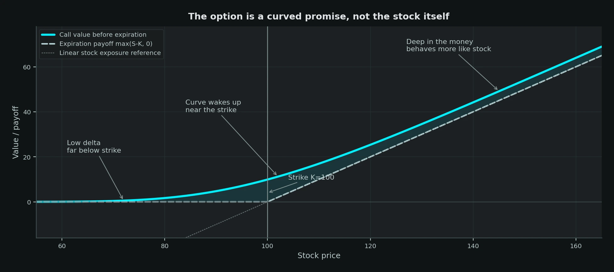
A call option value curve bending with stock price, compared with the expiration payoff and a linear stock exposure reference. — A call option is a curved promise: low sensitivity below the strike, faster response near the strike, and near-linear behavior when deep in the money.

A stock moves one-for-one with itself. A call option does not. When the stock is far below the strike, the option may barely move. Near the strike, it wakes up. Deep above the strike, it starts behaving more like the stock.

So the option is not just a forecast about the final stock price. It is a changing sensitivity to the stock price.

That sensitivity will become the central object.

We call it delta:

Δ = \frac{\partial V}{\partial S}

Here, $V (S, t)$ is the option value as a function of stock price $S$ and time $t$ .

Delta answers a local question:

If the stock moves a tiny bit right now, how much does the option value move?

Black-Scholes starts by taking that local question seriously.

The Tempting but Wrong Shortcut

The most natural first attempt is expectation.

Simulate many possible stock paths. Compute the call payoff on each path. Average the payoffs. Discount the average back to today.

That sounds reasonable.

But which average?

Under the real-world stock process, the drift is $μ$ :

d S_{t} = μ S_{t} d t + σ S_{t} d W_{t}

If we use $μ$ , we need to know the stock's expected return. That is already hard. Worse, the option is risky, so discounting its expected payoff should involve a risk premium. But whose risk premium? A pension fund's? A market maker's? A retail trader's? A bank's?

This was the historical trap.

Before Black, Scholes, and Merton, it was natural to think option pricing required an opinion about expected stock return and investor risk appetite. The Nobel Prize's 1997 explanation of their work emphasizes exactly this point: assigning the right risk premium was difficult because it depends on risk preferences that are hard to observe.

Black-Scholes escapes the trap by not starting with the expected payoff.

It starts with a hedge.

The Hedge Is the Trick

Suppose you own one option.

Its value is:

V (S, t)

Because the option reacts to the stock, you can offset that local reaction by trading the stock.

Create a portfolio:

Π = V - Δ S

That means:

long one option;
short $Δ$ shares of stock.

If $Δ$ is chosen correctly, a tiny stock move changes the option and the stock position by the same amount in opposite directions.

This does not mean the portfolio is safe forever.

Delta changes as the stock moves and time passes. A real hedge must be adjusted. That is why the Nobel explanation describes the composition of the stock-option portfolio as something that must gradually change as maturity approaches and the stock price changes.

But instant by instant, inside the idealized model, the hedge can cancel the random shock.

That is the heart of the argument.

Not the formula.

Not the normal distribution table.

The hedge.

Bring Back Itô

Now we need the same tool that powered the previous bridge post.

The stock follows GBM:

d S = μ S d t + σ S d W

The option is a function of the stock and time:

V = V (S, t)

Because $S$ is random, $V$ is random too. Itô's lemma tells us how $V$ changes:

d V = (\frac{\partial V}{\partial t} + μ S \frac{\partial V}{\partial S} + \frac{1}{2} σ^{2} S^{2} \frac{\partial ^{2} V}{\partial S ^{2}}) d t + σ S \frac{\partial V}{\partial S} d W

Read that slowly.

The first bracket is the time part. It accumulates with $d t$ .

The last term is the random part. It moves with $d W$ .

The option inherits randomness from the stock through:

σ S \frac{\partial V}{\partial S} d W

That is why delta matters. The coefficient of the random stock shock contains:

\frac{\partial V}{\partial S}

So set the hedge ratio equal to delta:

Δ = \frac{\partial V}{\partial S}

Now calculate the hedged portfolio:

Π = V - Δ S

Its change is:

d Π = d V - Δ d S

Substitute the option change and the stock change:

d Π = (\frac{\partial V}{\partial t} + μ S \frac{\partial V}{\partial S} + \frac{1}{2} σ^{2} S^{2} \frac{\partial ^{2} V}{\partial S ^{2}}) d t + σ S \frac{\partial V}{\partial S} d W - \frac{\partial V}{\partial S} (μ S d t + σ S d W)

Now the cancellation appears.

The random terms:

σ S \frac{\partial V}{\partial S} d W - \frac{\partial V}{\partial S} σ S d W = 0

The drift terms involving $μ$ cancel too:

μ S \frac{\partial V}{\partial S} d t - \frac{\partial V}{\partial S} μ S d t = 0

What remains is:

d Π = (\frac{\partial V}{\partial t} + \frac{1}{2} σ^{2} S^{2} \frac{\partial ^{2} V}{\partial S ^{2}}) d t

The expected stock return has disappeared.

That is the moment.

The stock drift drops out because the hedge is built from the same stock that creates the option's risk.

This is why Black-Scholes is not a forecast of the stock's expected return. It is a local replication argument. In the ideal model, the option's stock risk can be offset by trading the stock itself.

No-Arbitrage Finishes the Argument

We now have a hedged portfolio with no random $d W$ term:

Π = V - S \frac{\partial V}{\partial S}

and:

d Π = (\frac{\partial V}{\partial t} + \frac{1}{2} σ^{2} S^{2} \frac{\partial ^{2} V}{\partial S ^{2}}) d t

If this portfolio is locally risk-free, then in an arbitrage-free market it must earn the risk-free rate:

d Π = r Π d t

So:

(\frac{\partial V}{\partial t} + \frac{1}{2} σ^{2} S^{2} \frac{\partial ^{2} V}{\partial S ^{2}}) d t = r (V - S \frac{\partial V}{\partial S}) d t

Cancel $d t$ and rearrange:

\frac{\partial V}{\partial t} + \frac{1}{2} σ^{2} S^{2} \frac{\partial ^{2} V}{\partial S ^{2}} + r S \frac{\partial V}{\partial S} - r V = 0

That is the Black-Scholes partial differential equation.

It does not contain $μ$ .

It does contain:

the stock price ( $S$ );
time ( $t$ );
volatility ( $σ$ );
the risk-free rate ( $r$ );
the option's sensitivity to stock price ( $Δ$ );
the option's curvature with respect to stock price ( $Γ$ ).

The risk problem has become a pricing equation.

graph LR
    A["GBM stock path"] --> B["Option value V(S,t)"]
    B --> C["Ito expansion"]
    C --> D["Choose delta"]
    D --> E["Cancel dW"]
    E --> F["Risk-free local portfolio"]
    F --> G["Black-Scholes PDE"]

This is the part that often gets hidden when the formula is introduced first.

The formula is the solution.

The PDE is the machine.

The hedge is the engine.

The Boundary Condition Is the Contract

A PDE alone is not enough.

We also need to know what the option is worth at expiration.

For a European call option with strike $K$ and maturity $T$ :

C (S, T) = max (S_{T} - K, 0)

At maturity, there is no mystery. The option is worth its payoff.

Before maturity, the PDE tells us how that terminal payoff should be valued backward through time under the model assumptions.

Solving the PDE gives the familiar call formula:

C = S N (d_{1}) - K e^{- r (T - t)} N (d_{2})

where:

d_{1} = \frac{ln ( S / K ) + ( r + \frac{1}{2} σ ^{2} ) ( T - t )}{σ T - t}

and:

d_{2} = d_{1} - σ T - t

Here $N (\cdot)$ is the standard normal cumulative distribution function.

This is the line people memorize.

But if you memorize only this line, you miss the point.

The formula is not a mysterious spell for producing option prices. It is the closed-form answer to a very specific idealized problem:

the stock follows GBM;
volatility is constant;
the risk-free rate is known and constant;
trading is continuous;
there are no transaction costs or taxes;
the option is European;
the hedge can be adjusted perfectly.

Once those assumptions are in place, the formula follows.

Once those assumptions fail, the formula becomes a benchmark.

That benchmark is still valuable.

What the Formula Is Really Saying

The call price:

C = S N (d_{1}) - K e^{- r (T - t)} N (d_{2})

has two pieces.

The first piece:

S N (d_{1})

acts like the stock-linked part.

The second piece:

K e^{- r (T - t)} N (d_{2})

acts like the discounted strike-linked part.

The option value is the difference between those two weighted pieces.

That is useful, but the Greeks are often more revealing than the price itself.

Delta:

\frac{\partial V}{\partial S}

tells us how much stock exposure the option behaves like locally.

Gamma:

\frac{\partial ^{2} V}{\partial S ^{2}}

tells us how fast delta changes.

Theta:

\frac{\partial V}{\partial t}

tells us how the option changes as time passes.

Vega, usually written as sensitivity to volatility, tells us how much the option price changes when $σ$ changes.

Rho tells us sensitivity to the interest rate.

The Greeks are not decorative labels. They are the risk controls that fall out of the pricing machine. If the price is the answer, the Greeks are the operating manual.

This is why Black-Scholes remained useful even after everyone learned that market volatility is not constant. It gave traders a shared coordinate system:

price;
delta;
gamma;
theta;
vega;
implied volatility.

Real markets disagree with the model every day. But the disagreement is measurable.

That is the value of a baseline.

The Risk-Neutral Shortcut

There is another way to say the same thing.

After the hedge argument removes $μ$ , we can price the option as if the stock earns the risk-free rate under a special probability measure:

d S_{t} = r S_{t} d t + σ S_{t} d W_{t}^{Q}

Then the option value is the discounted expected payoff under that risk-neutral measure:

V (S, t) = e^{- r (T - t)} E^{Q} [payoff (S_{T}) ∣ S_{t} = S]

This sentence is powerful, but it can also mislead beginners.

Risk-neutral does not mean investors are risk neutral.

It does not mean the stock's real expected return is $r$ .

It means that, inside the arbitrage-free pricing framework, we can value the derivative using a transformed probability world where discounted tradable assets behave consistently with no-arbitrage pricing.

For the purpose of this series, keep the intuition simple:

The hedge removes the need to estimate $μ$ .

The risk-neutral expectation is the cleaned-up pricing language that results.

Why the Assumptions Matter

The Black-Scholes model assumes a world that is much cleaner than the one traders actually inhabit.

Real markets have transaction costs.

Trading is discrete.

Liquidity vanishes when it matters.

Volatility moves.

Prices jump.

Borrowing and lending rates differ.

Options can be American-style, path-dependent, barrier-triggered, callable, convertible, or embedded in messy corporate contracts.

The hedge is never adjusted continuously. Even if it could be, the act of hedging costs money and changes exposure.

So the model is wrong.

That is not the end of the story.

It is the beginning of professional quant finance.

When implied volatility changes by strike and maturity, the market is telling us constant $σ$ is not enough.

When a delta hedge loses money during a jump, the market is telling us continuous diffusion is not enough.

When short-dated options behave differently around earnings or macro events, the market is telling us time-homogeneous randomness is not enough.

When a Monte Carlo simulation is needed for an exotic payoff, the market is telling us the closed form is not enough.

Black-Scholes gives the clean case first. Then every real-world complication can be understood as a correction to the clean case.

That is why it survived.

The Takeaway

Black-Scholes is usually remembered as a formula.

That is too small.

The real idea is a chain of reasoning:

model the stock path;
view the option as a function of stock price and time;
use Itô's lemma to see how the option moves;
choose delta so the random stock shock cancels;
require the locally risk-free portfolio to earn the risk-free rate;
solve the resulting PDE with the option payoff as the boundary condition.

The expected stock return disappears because the hedge uses the stock itself to remove local stock risk.

That is the magic trick.

Except it is not magic.

It is accounting, calculus, and no-arbitrage tied together carefully.

And once you understand that, the next step becomes natural.

What happens when the payoff is too complicated for a clean formula?

What happens when the path matters, not just the final price?

What happens when the assumptions are still useful, but the closed form stops helping?

Then we return to simulation.

The next post is Monte Carlo option pricing.

Previous Posts in This Thread

From Itô to Black-Scholes: How Randomness Became a Pricing Engine builds the bridge from stochastic calculus into quant finance.
Geometric Brownian Motion in Python: The First Model Every Quant Learns turns the stock-price model into simulated paths and terminal distributions.
The Quiet Genius Who Made Randomness Calculable explains why Itô calculus is the hinge.
Bachelier's Revenge: The Forgotten Thesis of Modern Finance shows why finance entered the randomness story early.

References

Fischer Black and Myron Scholes, "The Pricing of Options and Corporate Liabilities", Journal of Political Economy, 1973.
Robert C. Merton, "Theory of Rational Option Pricing", The Bell Journal of Economics and Management Science, 1973.
Nobel Prize, The Prize in Economic Sciences 1997 - Press release, October 14, 1997.

Contents