The Quiet Genius Who Made Randomness Calculable
Kyoto, 1998.
An elderly mathematician stands before an audience and looks back over sixty years of probability theory. The title of his lecture is modest: My Sixty Years along the Path of Probability Theory. The man delivering it is modest too. Soft-spoken. Precise. Not the kind of scientific hero whose story gets told with explosions, rivalries, or grand public debates.
His name is Kiyosi Itô.
By the time he gives that lecture, the mathematical language he invented is already everywhere. It is inside option-pricing engines on Wall Street. It is inside models of noisy electrical circuits and chemical reactions. It is inside filtering systems that estimate position from imperfect sensors. It is inside stochastic control, population biology, statistical physics, and eventually the continuous-time view of diffusion models in machine learning.
And yet Itô's great achievement is easy to underestimate because it sounds, at first, like a technicality.
He defined a new kind of integral.
That sentence does not sound like the beginning of a revolution. It sounds like homework.
But this was not an ordinary integral. It was an integral designed for motion with no velocity, for signals with no slope, for paths that are continuous but so jagged that ordinary calculus cannot touch them. Brownian motion had been seen under a microscope, used in finance, explained by physics, and made rigorous by Norbert Wiener.
Itô gave it a calculus.
Monte Carlo made randomness computable. Wiener made Brownian paths rigorous. Itô made those paths calculable.
This is a new thread in the stochastic series. In earlier posts, we followed the story from Monte Carlo methods to Bachelier's forgotten finance thesis to Norbert Wiener's construction of continuous randomness and a practitioner's guide to SDEs.
Now we come to the quiet hinge in the story: the moment randomness stopped being only something to simulate and became something you could transform with rules.
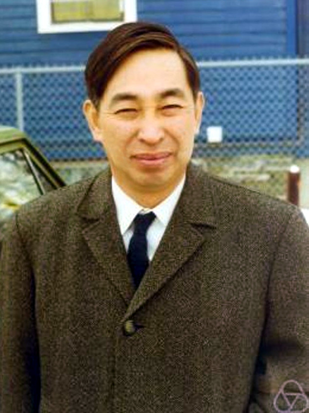
Konrad Jacobs, CC BY-SA 2.0 DE, via Wikimedia Commons
Contents
The Story So Far
It started, as this whole chain of ideas always seems to, with pollen.
In 1827, Robert Brown watched tiny particles suspended in water jitter unpredictably under a microscope. The motion was not smooth. It was not periodic. It did not seem to have a cause that could be isolated and removed. Brown did the careful work of ruling out biological explanations, but he could not explain what remained.
The nineteenth century had a problem. Classical mechanics described a deterministic universe. Brownian motion looked like nature refusing to behave that way.
Then the same random structure appeared somewhere stranger: the Paris stock market. In 1900, Louis Bachelier modeled price changes as a random walk in his thesis on speculation. He effectively wrote down Brownian-style mathematics before physicists had finished explaining Brownian motion itself.
Five years later, Einstein gave the physical explanation. The particle was not alive. It was being kicked from all sides by molecules too small to see. The random path became evidence for the atomic structure of matter.
Then Norbert Wiener made the object mathematically real. In 1923, he constructed what we now call the Wiener process: a probability measure on continuous paths. Brownian motion was no longer just a physical phenomenon or a financial metaphor. It was a rigorous mathematical object.
That should have been the end of the story.
It was not.
Wiener had built the house. But the tools of calculus still did not work inside it.
By the 1920s, Brownian motion existed mathematically. The problem was that ordinary calculus still had no idea what to do with it.
The issue is not that Brownian paths have jumps. They do not. A Brownian path is continuous. It moves without teleporting.
The issue is worse: it is continuous but almost surely nowhere differentiable. Zoom in and the path does not become a smooth curve. It remains rough. Zoom in again and the roughness is still there. There is no point where the path settles down enough to have an ordinary slope.
Classical calculus is built around slope. If there is no slope, the basic machinery starts to fail.
That was the gap Itô walked into.
A Young Mathematician in Wartime Japan
Kiyosi Itô was born on September 7, 1915, in what is now Inabe, Mie Prefecture, Japan. He studied mathematics at Tokyo Imperial University and entered probability at a time when the field was still becoming a modern discipline.
This matters. Probability today feels foundational. Every engineer talks about distributions, noise, inference, uncertainty, stochastic gradients, risk, sampling. But in the first half of the twentieth century, probability was still being rebuilt on rigorous foundations. Kolmogorov's axioms had appeared in 1933. Wiener's Brownian motion was only a decade older than that. Martingales, Markov processes, stochastic integration, stochastic differential equations: these were not settled tools sitting on a shelf. They were being invented.
Itô began his career in that unfinished world.
During the early 1940s, communication between Japanese mathematicians and the rest of the world was constrained by war, language, geography, and the basic difficulty of the subject itself. Itô was not working in the glamorous center of a large international program. He was building a theory in a field whose eventual applications were not yet obvious.
In 1944, while affiliated with Nagoya Imperial University, he published a short paper in the Proceedings of the Imperial Academy titled "Stochastic Integral". It was six pages long.
Six pages is not much room for a new branch of mathematics.
But the central idea was there: define integration with respect to a stochastic process in a way that respects time, information, and the fact that Brownian paths are not differentiable.
Seven years later, in 1951, he published "On a Formula Concerning Stochastic Differentials", giving the formula that would become known as Itô's lemma.
That formula is the stochastic chain rule.
The phrase sounds small. It is not.
Why Ordinary Calculus Breaks
Imagine a smooth curve. At any point, you can zoom in far enough and the curve begins to look like a straight line. That is the local idea behind a derivative. The derivative is the slope of that line.
Interactive intuition
Zoom until the curve becomes a line. Then try Brownian motion.
A derivative is local. A smooth curve starts looking linear when the window gets small. A Brownian-style path does not settle down the same way: zooming reveals more roughness instead of a stable slope.
Brownian motion refuses this bargain.
It is continuous, so it does not jump. But its local behavior is too erratic to flatten into a line. The closer you look, the more jagged motion you find. A Brownian path is not a bad smooth curve. It is a fundamentally different kind of object.
The technical reason is hidden in the scaling.
For a small time step , a Brownian increment behaves like:
That is already strange. In ordinary calculus, small changes scale like . Brownian changes scale like the square root of time.
Now square the increment:
This is where the world changes.
In ordinary calculus, second-order terms like vanish so quickly that we ignore them. That is why the usual chain rule works the way it does. But with Brownian motion, the square of the random increment is not negligible. It contributes at the same order as time itself.
So when you apply a nonlinear function to a Brownian-driven process, curvature matters. Randomness interacts with the second derivative.
That is the source of Itô's correction term.
The Itô correction is not a trick. It is the price of doing calculus on paths whose squared wiggles accumulate into time.
For a stochastic process written in the form:
Itô's lemma says that a function evolves as:
If you are seeing this for the first time, focus on the extra term:
That term is the signature of Itô calculus.
It says that a nonlinear function of a noisy process does not simply follow the ordinary chain rule. The process's volatility and the function's curvature create an additional drift.
Randomness has geometry.
The Most Expensive Correction Term in Finance
The cleanest example is geometric Brownian motion, the model that sits under Black-Scholes:
Here is an asset price, is expected return, and is volatility.
Now ask a simple question: how does evolve?
In ordinary calculus, you might expect:
That would give:
But that is wrong.
Itô's lemma adds the curvature correction:
There it is: .
Volatility lowers the growth rate of log wealth. The average price and the average log price do not move the same way. If you have ever heard the phrase "volatility drag," this is the calculus hiding underneath it.
This correction term is not academic bookkeeping. It is part of the machinery that made modern quantitative finance possible. Black, Scholes, and Merton used Itô calculus to reason about option prices under continuous hedging. The model has idealized assumptions, and real markets violate many of them, but the conceptual shift was permanent.
Before Itô, randomness in markets could be described.
After Itô, randomness in markets could be transformed.
Black-Scholes matters not because markets are perfectly lognormal, but because Itô calculus taught finance how to compute with uncertainty.
That is why the story of Itô is not just a story about probability theory. It is a story about turning uncertainty into an engineering object.
The Calculus of Not Knowing the Future
One of Itô's most important modeling choices is easy to miss.
The Itô integral uses information from the present, not the future. In a discrete approximation, the integrand is evaluated at the left endpoint of each time interval. That means the value you multiply by the next random shock is based on what you know before the shock arrives.
That sounds obvious.
It is also profound.
A trading strategy cannot depend on tomorrow's price. A filter cannot depend on next week's sensor reading. A controller cannot choose today's action using a future state it has not observed yet. A simulation step should update from the current state into the next random increment, not cheat by peeking ahead.
Itô calculus bakes this discipline into the mathematics.
That is why it is so natural for finance, filtering, control, and simulation. It respects the direction of information flow.
There is another stochastic calculus, the Stratonovich calculus, that uses a midpoint-style interpretation and preserves the ordinary chain rule. It is often useful in physics, especially when white noise is the limiting form of smoother noise.
This is not a fight between right and wrong.
It is a choice about what the equation means.
Itô is the calculus of non-anticipating systems. Stratonovich is the calculus of smooth-noise limits. Same noise symbol. Different accounting.
We will come back to that in a later post, because it is one of the most common places where stochastic modeling goes wrong.
For now, the important point is simple: Itô's definition did not merely solve a technical problem. It matched the structure of real decisions under uncertainty.
Itô calculus is not just about randomness. It is about randomness arriving in time, one shock after another, with no permission to read the future.
Why the World Needed This
Once Itô calculus existed, a new kind of modeling language became available.
You could write:
and mean something precise.
The first term, , is drift: the systematic tendency of the system. The second term, , is diffusion: the random shock scaled by the current state and time.
That compact expression can describe very different worlds.
In physics, it describes a particle pulled by friction and kicked by unresolved microscopic collisions.
In finance, it describes a price with expected return and volatility.
In biology, it describes a population whose average growth is shaped by birth and death, but whose survival is threatened by unlucky paths.
In engineering, it describes a hidden state evolving under process noise while sensors deliver imperfect observations.
In machine learning, the same continuous-time vocabulary appears in score-based generative models: forward processes that turn data into noise, reverse processes that learn how to turn noise back into data.
The power is not that every one of these systems is literally the same. The power is that the same grammar can express them.
Drift. Diffusion. Brownian shocks. Information flow. Transformation rules. Simulation schemes.
Itô gave that grammar a chain rule.
Recognition Came Late, But It Came
Itô's work eventually became impossible to ignore.
He spent much of his academic career at Kyoto University and also held visiting positions abroad, including at Aarhus and Cornell. In 1998, he received the Kyoto Prize in Basic Sciences. The Kyoto Prize citation recognized his fundamental contribution to stochastic analysis and noted the reach of stochastic differential equations across physics, engineering, biology, and economics.
In 2006, he received the first Carl Friedrich Gauss Prize for Applications of Mathematics from the International Mathematical Union. That award matters because it is specifically about mathematics whose influence extends into the applied world.
Itô was ninety years old.
The timing feels appropriate. Some mathematical ideas announce their importance immediately. Others spread quietly until whole industries depend on them.
Itô calculus is the second kind.
If you use a risk model, simulate noisy dynamics, estimate hidden state, price derivatives, analyze stochastic optimization, or study diffusion models, you are living downstream of that six-page 1944 paper.
Not directly in every line of code. Not always consciously. But structurally.
The modern world is full of systems that cannot be understood by their average path alone. They must be understood as distributions over paths. Itô calculus is one of the core languages for doing that.
The Real Lesson
There is a tempting but wrong way to summarize Itô's achievement:
He made Brownian motion differentiable.
He did not.
Brownian motion remains jagged. It remains nowhere differentiable almost surely. Itô did something more subtle and more powerful: he stopped trying to force randomness into the shape of ordinary calculus.
He built a calculus that respected the roughness.
That is the deeper lesson for anyone who builds models.
Bad modeling often begins by smoothing away the inconvenient part of reality. Average the noise. Linearize the behavior. Pretend uncertainty is just an error bar around a deterministic core. Sometimes that works. Often it does not.
Itô's work says: do not erase the randomness too early. Give it rules. Track how it accumulates. Understand how it changes nonlinear transformations. Preserve the direction of information. Then compute.
That is why this story belongs in a data and AI architecture series, not only in a math history series.
Modern systems operate under uncertainty. Users behave unpredictably. Markets move. Sensors drift. Models hallucinate. Training runs follow noisy gradients. Generative models reverse carefully designed corruption processes. The question is not whether randomness exists.
The question is whether your architecture has a language for it.
Itô did not smooth randomness into calculus. He rebuilt calculus so randomness could remain rough.
In the next post, we will open the engine and look at the exact place ordinary calculus fails: the chain rule. The whole mystery turns on one small fact:
That line looks impossible the first time you see it.
It is also where stochastic calculus begins.
Sources and Further Reading
- Kiyosi Itô, "Stochastic Integral", Proceedings of the Imperial Academy, 1944.
- Kiyosi Itô, "On a Formula Concerning Stochastic Differentials", Nagoya Mathematical Journal, 1951.
- Kyoto Prize, Kiyosi Itô laureate profile.
- International Mathematical Union, Gauss Prize 2006: Kiyosi Itô.
- Desmond Higham, "An Algorithmic Introduction to Numerical Simulation of Stochastic Differential Equations", 2001.