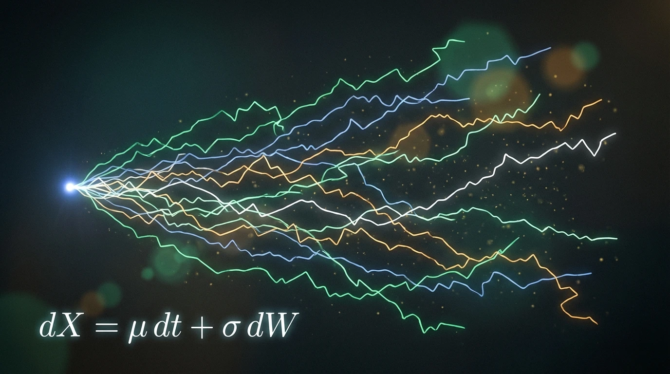
When Randomness Met Calculus: A Practitioner's Guide to Stochastic Differential Equations
In the previous post in this series, we met Kiyosi Itô — a Japanese mathematician working in near-isolation during World War II, building a rigorous language for processes that were continuous in time but genuinely, irreducibly random. His work extended calculus into territory where ordinary derivatives don't exist, where paths are too jagged to have a slope at any point.
We left Itô's contribution as a historical footnote. It isn't one.
Today, Itô calculus is the backbone of quantitative finance, statistical physics, computational biology, and machine learning. Every time a risk system prices an option, every time an epidemic model accounts for random superspreading, every time a GPS filter estimates your position despite noisy sensors — there is a stochastic differential equation running under the hood.
This post is about learning to read and write that language.
We'll build from first principles — no PhD required — and end with working Python code that simulates three real systems: a particle being battered by thermal noise, a population teetering on the edge of extinction, and a stock price wandering through an uncertain market.
This is Part 3 of the Monte Carlo series. Start with Part 1 for hands-on Monte Carlo integration, then Part 2 for the fascinating human history. Here we get technical — but the story stays alive.
Contents
Why Ordinary Calculus Isn't Enough
Classical differential equations describe how things change over time. Newton's second law, , can be rewritten as:
Given the force and the initial velocity, you can predict the future velocity at every moment. The trajectory is smooth. Deterministic. If you know the present exactly, you know the future exactly.
This is a beautiful theory. It is also frequently wrong.
Consider what Robert Brown saw in 1827: pollen grains in water, moving in erratic, unpredictable paths. Not smooth curves — jagged zigzags that changed direction thousands of times per second. An ODE cannot capture this. Any solution to an ODE has a well-defined slope everywhere. Brownian paths don't.
Or consider a bacteria colony of 50 individuals. At any moment, one bacterium might divide (birth) or die at random. The colony size tomorrow isn't determined by today's size alone — it depends on the random outcomes of hundreds of individual events. A smooth curve through the middle of those outcomes misses what's actually happening.
An ordinary differential equation says: given the present, the future is fixed. A stochastic differential equation says: given the present, the future is a distribution.
The fundamental difference between an ODE and an SDE is the addition of a noise term — a mathematical object that injects genuine, unpredictable randomness into the equation at every instant.
The tool we need is a Wiener process (also called Brownian motion): a continuous random function where:
- Increments for follow a normal distribution with mean 0 and variance
- Non-overlapping increments are independent — the future does not remember the past
This process exists, but its paths are nowhere differentiable. You cannot compute in the ordinary sense. Itô's great insight was developing a consistent calculus for functions of anyway.
The Anatomy of a Stochastic Differential Equation
The general form of an Itô SDE for a scalar process is:
This compact notation contains everything. Let's unpack it symbol by symbol.
| Symbol | Name | What It Means |
|---|---|---|
| State | The quantity we're tracking — position, population size, stock price | |
| Increment | The infinitesimally small change in over a tiny time window | |
| Drift | The deterministic tendency — where "wants" to go on average | |
| Time increment | An infinitesimally small step forward in time | |
| Diffusion | How strongly the randomness affects (larger = more noise) | |
| Wiener increment | A draw from — pure randomness scaled by time |
The equation reads: "The change in X over a tiny instant equals its systematic drift plus a random shock proportional to ."
The Crucial Strangeness of
In ordinary calculus, when is small, is negligibly small and we drop it. This is why second-order terms vanish in Taylor expansions.
With Brownian motion, something different happens. Since , we have:
The square of the random increment is not negligible — it is exactly . This means second-order terms involving survive in calculations. This is the source of Itô's correction term (Itô's lemma), which makes stochastic calculus fundamentally different from ordinary calculus.
You don't need to master Itô's lemma to simulate SDEs. But knowing this strangeness exists helps you understand why naive intuition sometimes fails.
Three Worlds, One Language
The same equation, , models radically different phenomena depending on how and are defined. Here are three of the most important instantiations.
Physics: The Langevin Equation
Edinburgh, 1827. The pollen grains are dancing.
We now know why. At room temperature, water molecules are in constant, violent thermal motion — striking a pollen grain roughly times per second. The net effect of all those collisions is effectively random: the particle receives random kicks from all directions, producing the erratic motion Brown documented.
French physicist Paul Langevin (1908) described this with what is now called the Langevin equation:
Where:
- is the particle's velocity
- is the friction coefficient — the drag from the fluid that resists motion
- is the noise strength — the intensity of thermal kicks
- is the Wiener increment — the random thermal force
The drift term says: the faster you move, the more the fluid slows you down. The diffusion term says: random molecular collisions are constantly kicking you.
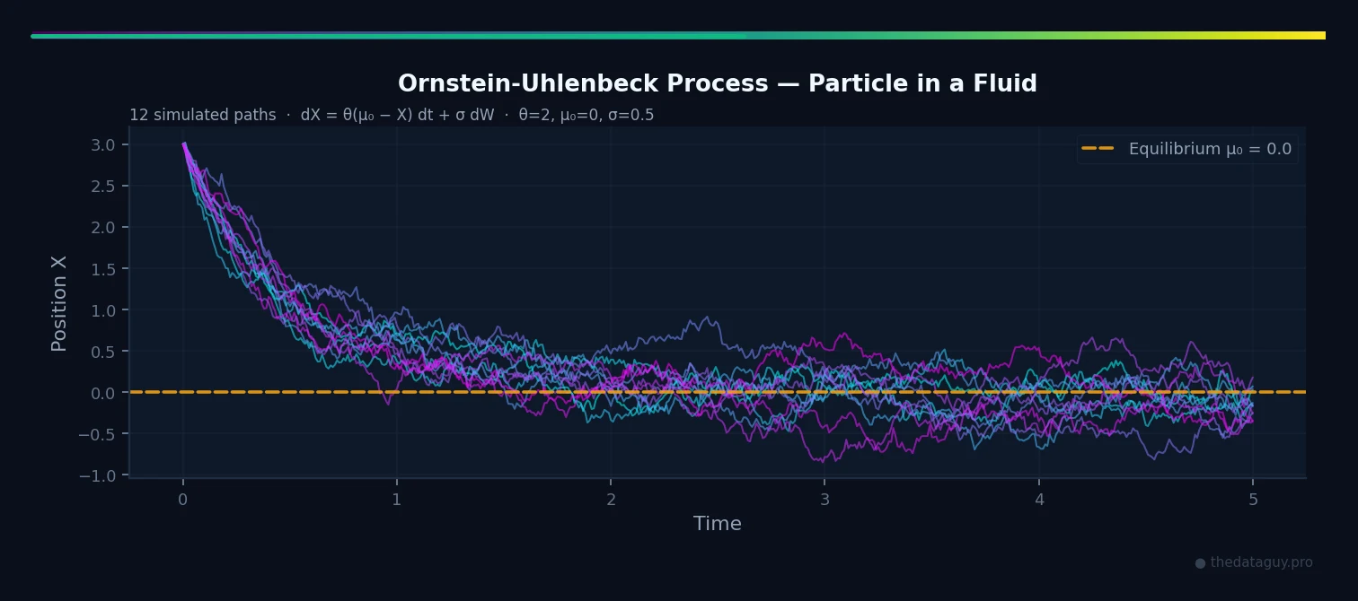
This is also called the Ornstein-Uhlenbeck (OU) process when we model position around a mean :
- : mean reversion rate — how strongly the process is pulled back toward the center
- : the equilibrium — the position or value the process tends to return to
- : noise amplitude
The OU process is one of the most useful SDEs in science precisely because of mean reversion — it describes any system that fluctuates around a stable equilibrium. Molecular velocities. Ion channel conductance. Body temperature. These systems don't wander away forever; they stay near a fixed point, with random fluctuations.
Biology: Stochastic Population Dynamics
Classical ecology uses the logistic growth equation to model how a population grows toward a carrying capacity :
This is clean and deterministic. But real populations experience environmental stochasticity — random droughts, disease outbreaks, unpredictable food supplies. For small populations (endangered species, bacterial colonies in a micro-environment), demographic stochasticity matters too: each individual birth and death is a discrete random event.
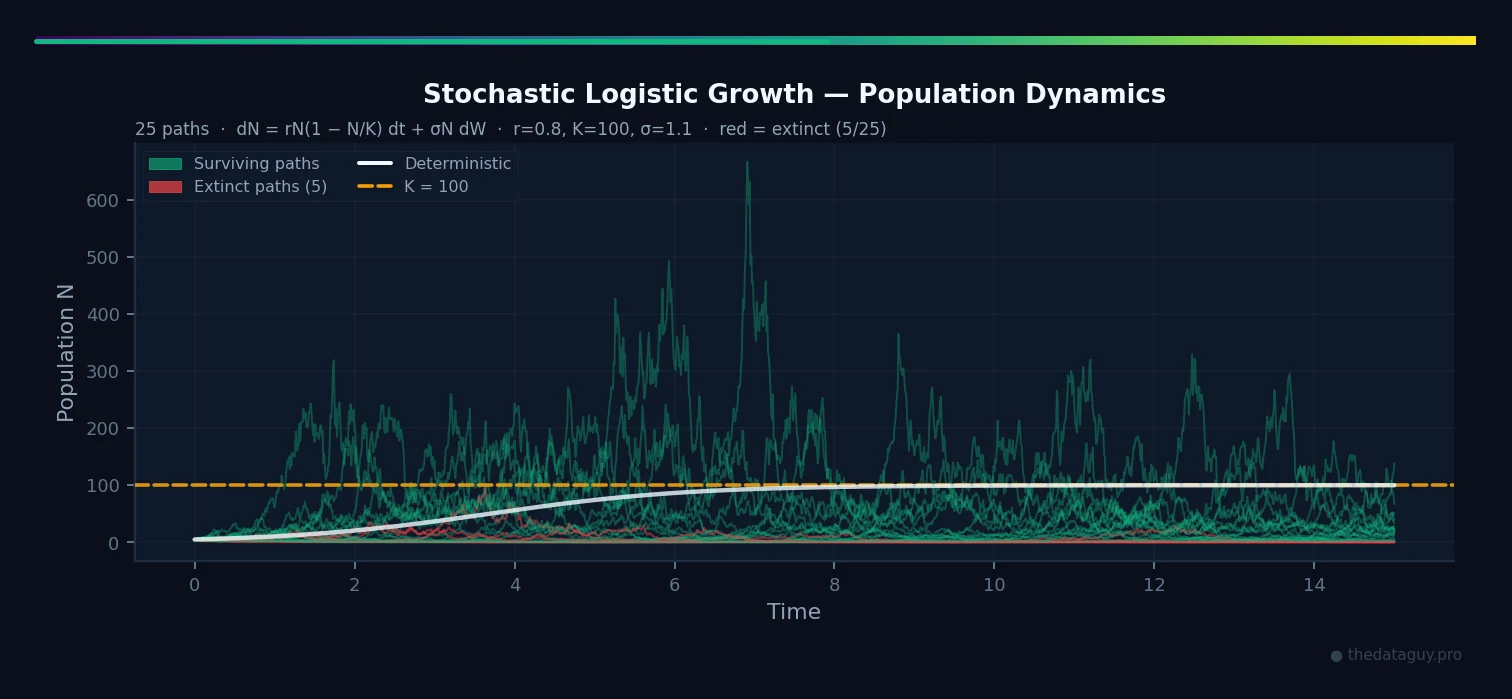
The stochastic logistic equation captures this:
Where:
- : intrinsic growth rate
- : carrying capacity (the population ceiling)
- : environmental noise intensity
- : multiplicative noise — the randomness scales with population size (a small colony is more vulnerable to proportional shocks than a large one)
The crucial difference from the deterministic version: even if the deterministic model predicts eventual recovery to , the stochastic version allows extinction — the population can hit zero and never recover. This has profound implications for conservation biology. A species that "should" survive based on mean dynamics can still go extinct through a sequence of unlucky years.
The stochastic logistic model teaches a lesson no deterministic model can: mean dynamics are not destiny. Variance kills.
Finance: Geometric Brownian Motion
In 1900, Louis Bachelier proposed that stock prices follow a random walk. Einstein independently derived the mathematics of Brownian motion five years later. Eventually, the two threads merged.
The Geometric Brownian Motion (GBM) model for asset prices is:
Where:
- : current asset price
- : drift — the expected return (average percentage growth per unit time)
- : volatility — the standard deviation of returns (how noisy the price is)
- : multiplicative noise — the random shocks are proportional to the current price
Why multiplicative? Because a $10 move on a $10 stock is catastrophic; a $10 move on a $1,000 stock is a rounding error. Price shocks scale with price level.
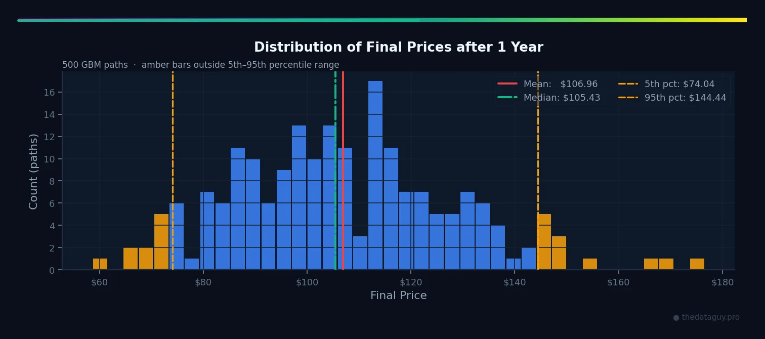
GBM is the foundation of the Black-Scholes option pricing formula (Nobel Prize, 1997) — the single most influential equation in quantitative finance. The formula gives the "fair" price for an options contract, and its derivation relies on simulating thousands of GBM paths to see how often they end in the money.
GBM has known flaws (real markets have fat tails, volatility clusters, jumps), but as a first model it is remarkably powerful — and it is exactly what we will implement.
The Euler-Maruyama Method
We have the continuous equation. Now we need to actually simulate it on a computer.
The Euler-Maruyama (EM) method, developed by Gisiro Maruyama in 1955, is the simplest and most direct approach. It is the stochastic equivalent of the classical Euler method for ODEs: discretize time into small steps, and advance the solution one step at a time.
Given , the EM discretization is:
Where:
- : the time step size (small, but finite)
- : a standard normal random number, drawn fresh at each step
- : this approximates — the discretized Wiener increment
Why and not just ? Because the variance of equals (from the Wiener process definition), so the standard deviation is . This is the stochastic calculus difference in action: the noise term shrinks as , not , which means it dominates the drift for small .
The algorithm:
1. Set initial state X₀, time step Δt, total time T
2. For each step n = 0, 1, ..., T/Δt:
   a. Draw Z ~ N(0,1)
   b. X_{n+1} = X_n + μ(X_n, t_n)·Δt + σ(X_n, t_n)·√Δt·Z
3. Return the path {X₀, X₁, ..., X_N}
Each run of this algorithm gives one sample path — one possible trajectory the system could follow. To understand the system's behavior, we run many paths and study their distribution.
Python: A Universal SDE Simulator
Let's implement this. We'll build a clean, reusable EM solver and use it for all three systems.
import numpy as np
import matplotlib.pyplot as plt
from typing import Callable

def euler_maruyama(
    drift: Callable[[float, float], float],
    diffusion: Callable[[float, float], float],
    x0: float,
    t_start: float,
    t_end: float,
    dt: float,
    n_paths: int = 1,
    seed: int | None = None
) -> tuple[np.ndarray, np.ndarray]:
    """
    Simulate an Itô SDE using the Euler-Maruyama method.

    dX = drift(X, t) dt + diffusion(X, t) dW

    Parameters
    ----------
    drift       : function(X, t) -> float  —  the μ(X,t) term
    diffusion   : function(X, t) -> float  —  the σ(X,t) term
    x0          : initial state X(t_start)
    t_start     : start time
    t_end       : end time
    dt          : time step size (smaller = more accurate)
    n_paths     : number of independent sample paths to simulate
    seed        : optional random seed for reproducibility

    Returns
    -------
    t           : 1D array of time points, shape (N+1,)
    X           : 2D array of paths, shape (n_paths, N+1)
    """
    if seed is not None:
        np.random.seed(seed)

    t = np.arange(t_start, t_end + dt, dt)
    N = len(t)
    X = np.zeros((n_paths, N))
    X[:, 0] = x0

    sqrt_dt = np.sqrt(dt)

    for i in range(N - 1):
        x_current = X[:, i]
        t_current = t[i]

        # Draw n_paths standard normal random variables at once
        Z = np.random.standard_normal(n_paths)

        # Euler-Maruyama step
        X[:, i + 1] = (
            x_current
            + drift(x_current, t_current) * dt
            + diffusion(x_current, t_current) * sqrt_dt * Z
        )

    return t, X
Now let's apply this to each of our three systems.
System 1: Ornstein-Uhlenbeck (Physics — Particle in a Fluid)
# OU Process parameters
theta = 2.0   # mean reversion rate (how fast the particle returns to center)
mu_0  = 0.0   # equilibrium position
sigma = 0.5   # thermal noise strength

# Define drift and diffusion functions for OU
def ou_drift(x, t):
    return theta * (mu_0 - x)

def ou_diffusion(x, t):
    return sigma   # constant: noise is independent of position

# Simulate
t, X_ou = euler_maruyama(
    drift=ou_drift,
    diffusion=ou_diffusion,
    x0=3.0,       # particle starts far from equilibrium
    t_start=0.0,
    t_end=5.0,
    dt=0.01,
    n_paths=10,
    seed=42
)

# Plot
fig, ax = plt.subplots(figsize=(10, 4))
for path in X_ou:
    ax.plot(t, path, alpha=0.4, linewidth=0.8, color='steelblue')
ax.axhline(mu_0, color='red', linestyle='--', linewidth=1.5, label=f'Equilibrium μ₀={mu_0}')
ax.set_title('Ornstein-Uhlenbeck Process — Particle in a Fluid')
ax.set_xlabel('Time')
ax.set_ylabel('Position X')
ax.legend()
plt.tight_layout()
plt.show()
You should see all 10 paths starting at position 3 (far from equilibrium) and being pulled back toward 0, while continuing to fluctuate randomly around it. The mean reversion rate means the particle returns to center in roughly time units — after that, it's thermal noise all the way.
System 2: Stochastic Logistic Growth (Biology — Population Dynamics)
# Stochastic logistic parameters
r     = 0.8    # intrinsic growth rate
K     = 100.0  # carrying capacity
sigma_bio = 0.15  # environmental stochasticity

def logistic_drift(N, t):
    return r * N * (1.0 - N / K)

def logistic_diffusion(N, t):
    # Multiplicative noise: proportional to current population
    return sigma_bio * N

# Simulate from a small initial population
t, N_paths = euler_maruyama(
    drift=logistic_drift,
    diffusion=logistic_diffusion,
    x0=5.0,       # small initial population (5 individuals)
    t_start=0.0,
    t_end=15.0,
    dt=0.01,
    n_paths=30,
    seed=123
)

# Some paths may go negative — clip to 0 (extinction)
N_paths = np.clip(N_paths, 0, None)

# Count extinctions
n_extinct = np.sum(N_paths[:, -1] < 1.0)

fig, axes = plt.subplots(1, 2, figsize=(14, 4))

# Left: all paths
for path in N_paths:
    color = 'crimson' if path[-1] < 1.0 else 'forestgreen'
    axes[0].plot(t, path, alpha=0.3, linewidth=0.8, color=color)
axes[0].axhline(K, color='black', linestyle='--', linewidth=1.5, label=f'Carrying capacity K={K}')
axes[0].set_title(f'Stochastic Logistic Growth (30 paths)\n{n_extinct} extinctions in red')
axes[0].set_xlabel('Time')
axes[0].set_ylabel('Population N')
axes[0].legend()

# Right: distribution at final time
final_pops = N_paths[:, -1]
axes[1].hist(final_pops[final_pops > 1], bins=15, color='forestgreen', alpha=0.7, label='Surviving')
if n_extinct > 0:
    axes[1].axvline(0, color='crimson', linewidth=2, label=f'Extinct ({n_extinct})')
axes[1].set_title('Final Population Distribution (t=15)')
axes[1].set_xlabel('Final Population N')
axes[1].set_ylabel('Count')
axes[1].legend()

plt.tight_layout()
plt.show()

print(f"Surviving populations — Mean: {final_pops[final_pops > 1].mean():.1f}, "
      f"Std: {final_pops[final_pops > 1].std():.1f}")
print(f"Extinction rate: {n_extinct/len(N_paths)*100:.1f}%")
This is where SDEs teach something profound. The deterministic logistic model starting from always reaches . But the stochastic model occasionally kills the population before it can establish itself. Run many simulations and you can estimate the extinction probability — something a purely deterministic model cannot do.
System 3: Geometric Brownian Motion (Finance — Asset Prices)
# GBM parameters
mu_fin    = 0.08   # 8% annual drift (expected return)
sigma_fin = 0.20   # 20% annual volatility
S0        = 100.0  # initial price ($100)

def gbm_drift(S, t):
    return mu_fin * S

def gbm_diffusion(S, t):
    return sigma_fin * S

# Simulate over 1 year (252 trading days)
t, S_paths = euler_maruyama(
    drift=gbm_drift,
    diffusion=gbm_diffusion,
    x0=S0,
    t_start=0.0,
    t_end=1.0,
    dt=1/252,    # daily steps
    n_paths=500,
    seed=7
)

# Analytical mean path: S₀ · exp(μ·t)
analytical_mean = S0 * np.exp(mu_fin * t)

fig, axes = plt.subplots(1, 2, figsize=(14, 4))

# Left: sample of 50 paths
for path in S_paths[:50]:
    axes[0].plot(t, path, alpha=0.2, linewidth=0.5, color='royalblue')
axes[0].plot(t, analytical_mean, color='red', linewidth=2, linestyle='--',
             label=f'E[S(t)] = S₀·e^(μt)')
axes[0].set_title('GBM: 50 Simulated Stock Paths')
axes[0].set_xlabel('Time (years)')
axes[0].set_ylabel('Price ($)')
axes[0].legend()

# Right: distribution of final prices (500 paths)
final_prices = S_paths[:, -1]
axes[1].hist(final_prices, bins=40, color='royalblue', alpha=0.7, edgecolor='white')
axes[1].axvline(final_prices.mean(), color='red', linestyle='--',
                linewidth=2, label=f'Mean: ${final_prices.mean():.2f}')
axes[1].axvline(np.percentile(final_prices, 5), color='orange', linestyle='--',
                linewidth=1.5, label=f'5th pct: ${np.percentile(final_prices, 5):.2f}')
axes[1].axvline(np.percentile(final_prices, 95), color='orange', linestyle='--',
                linewidth=1.5, label=f'95th pct: ${np.percentile(final_prices, 95):.2f}')
axes[1].set_title('Distribution of Final Prices (500 paths, 1 year)')
axes[1].set_xlabel('Final Price ($)')
axes[1].set_ylabel('Count')
axes[1].legend()

plt.tight_layout()
plt.show()

print(f"GBM after 1 year (500 paths):")
print(f"  Starting price:    ${S0:.2f}")
print(f"  Mean final price:  ${final_prices.mean():.2f}  (theoretical: ${analytical_mean[-1]:.2f})")
print(f"  Median:            ${np.median(final_prices):.2f}")
print(f"  5th percentile:    ${np.percentile(final_prices, 5):.2f}  (Value at Risk boundary)")
print(f"  95th percentile:   ${np.percentile(final_prices, 95):.2f}")
print(f"  Probability > $100: {(final_prices > 100).mean()*100:.1f}%")
Notice something counterintuitive: the mean final price ($\approx $108$) is higher than the median ($\approx $105$). This asymmetry is a hallmark of log-normal distributions — GBM's final price follows a log-normal, not a normal. A few paths that shoot up dramatically drag the mean above the median. This is why "average return" and "most likely outcome" are not the same thing in financial modeling.
![Geometric Brownian Motion: 15 sample stock price paths over 1 year with red analytical mean E[S(t)] = S₀·e^(μt), starting at $100](/images/2026/04/stochastic-differential-equations-practitioners-guide/chart-gbm-paths.webp)
⚠️ Educational Disclaimer: The Geometric Brownian Motion example above — including the simulated stock paths, drift rate (μ = 8%), volatility (σ = 20%), and price distributions — is provided solely for mathematical and educational illustration of stochastic differential equations. It does not constitute financial advice, investment recommendations, or a prediction of any real security's future performance. Past statistical properties of financial markets are not indicative of future results. Real investment decisions involve risks, regulatory considerations, and personal circumstances that this model does not capture. Always consult a qualified financial professional before making investment decisions.
Convergence and When Euler-Maruyama Is Good Enough
The EM method has strong order 0.5 convergence: as the time step decreases, the path-wise error decreases as .
To reduce error by 10×, you need 100× smaller time steps. This is slower than classical Euler (which is order 1), but it is the cost of dealing with genuinely rough paths.
For most practical applications — pricing derivatives, simulating population dynamics, modeling particle diffusion — the EM method is sufficient. Here's a rule of thumb:
| Use case | Typical | Adequate? |
|---|---|---|
| Illustrative simulation | 0.01 – 0.001 | ✅ Yes |
| Financial option pricing | 1/252 (daily) to 1/1000 | ✅ Usually |
| High-precision physics | < 1e-4 | ⚠️ Check convergence |
| Stiff SDEs (large or $\sigma$) | Needs care | ❌ Use implicit methods |
A quick convergence test is always worth running: halve and check whether your quantity of interest (mean, variance, option price) changes significantly. If it doesn't, you're in the convergence regime.
# Strong convergence using shared Brownian paths (common random numbers).
# GBM exact solution: S(T) = S0 · exp((μ − σ²/2)·T + σ·W(T))
# We feed the same Brownian increments to both EM and the exact formula,
# then measure E[|S_EM(T) − S_exact(T)|] — path-wise error, no sampling noise.

rng = np.random.default_rng(42)
n_paths_conv = 10_000
dt_values = [0.1, 0.05, 0.02, 0.01, 0.005, 0.001]
errors = []

for dt in dt_values:
    N_steps = int(1.0 / dt)
    dW = rng.normal(0, np.sqrt(dt), size=(n_paths_conv, N_steps))
    W_T = dW.sum(axis=1)

    S_exact = S0 * np.exp((mu_fin - 0.5*sigma_fin**2)*1.0 + sigma_fin*W_T)
    S_em = np.full(n_paths_conv, S0, dtype=float)
    for i in range(N_steps):
        S_em = S_em + mu_fin*S_em*dt + sigma_fin*S_em*dW[:, i]

    errors.append(np.mean(np.abs(S_em - S_exact)))

fig, ax = plt.subplots(figsize=(7, 4))
ax.loglog(dt_values, errors, 'o-', color='royalblue', label='EM strong error')
ref = [errors[0] * np.sqrt(dt / dt_values[0]) for dt in dt_values]
ax.loglog(dt_values, ref, '--', color='gray', label='O(√Δt) reference')
ax.set_xlabel('Time step Δt')
ax.set_ylabel('E[|S_EM(T) − S_exact(T)|]')
ax.set_title('Euler-Maruyama Strong Convergence (GBM)')
ax.legend()
plt.tight_layout()
plt.show()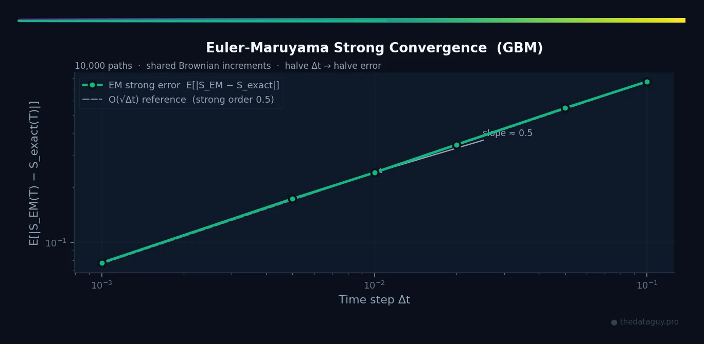
What SDEs Unlock
Mastering even basic SDE simulation opens up a large toolbox:
Uncertainty quantification. Instead of a single prediction, you get a distribution of outcomes. The 5th and 95th percentiles of your simulation are honest uncertainty bounds, not guesses.
Rare event estimation. What is the probability this population goes extinct? What's the chance this portfolio loses more than 20% in a year? Run enough paths and count.
Model calibration. You can fit and to real data (by matching the observed mean and variance of increments) and then extrapolate the model's implications.
Connecting to MCMC. Markov Chain Monte Carlo — the subject of a future post in this series — can be understood as a cleverly designed SDE being used to sample from a target distribution. The Langevin MCMC sampler literally uses the OU process as its sampling engine.
Machine learning. Diffusion models — the technology behind Stable Diffusion, DALL-E, and modern generative AI — are SDEs run in reverse. Data is corrupted by adding Gaussian noise (forward SDE), and the model learns to reverse that process (reverse-time SDE). Every image generated by a diffusion model involves thousands of EM steps.
From Itô's wartime notebooks to the images generated by DALL-E — the chain of ideas is direct, unbroken, and humbling.
What Comes Next
We've now crossed a significant threshold. We started this series by computing an integral with random sampling (Part 1). We learned the human story of how that idea was born (Part 2). Now we can simulate continuous-time random processes that describe the physical world.
The next step in the series goes deeper into the machinery: Markov Chain Monte Carlo (MCMC) — a technique for sampling from complex, high-dimensional probability distributions that are otherwise impossible to work with. MCMC is the workhorse of Bayesian statistics, computational biology, and modern machine learning.
The connection to what we've done here is tight: MCMC is, at its core, an SDE being used backwards — not to simulate a system, but to explore a distribution by constructing a random walk that settles into it.
If you've followed this series, you're ready.
Full notebook with all the code above: The complete, runnable Jupyter notebook for this post is available on GitHub.
Get in Touch
Stochastic differential equations sit at the crossroads of mathematics, physics, biology, and finance — and they're increasingly relevant in machine learning. If this post helped demystify them, or if you're applying SDEs to a real problem and want to talk through the modeling choices, I'd love to hear from you.
Connect with me:
- 📧 Email: [email protected]
- 🐦 Twitter/X: @TheDataGuyPro
- 💼 LinkedIn: Muhammad Afzaal
- 💻 GitHub: @mafzaal
- 🎥 YouTube: @TheDataGuyPro
- 🎧 Podcast: TheDataGuy Show
Whether you're modeling epidemic dynamics, pricing exotic derivatives, or building a diffusion model for generative AI — if randomness is at the core of your problem, I'd love to discuss it.
Related Posts
The Monte Carlo Series:
- From Symbolic Math to Random Sampling: Mastering Integral Calculations with Python — Part 1: hands-on Monte Carlo integration
- From Pollen Grains to Nuclear Bombs: The Astonishing Story of Monte Carlo Methods — Part 2: the human history of randomness
Mathematical Foundations:
- SymPy and Generative AI for Mathematical Reasoning — Symbolic math as a complement to numerical simulation
Data Science & ML:
- Chronos-2: The Evolution from Univariate to Universal Time Series Forecasting — Probabilistic forecasting at scale
- Truth is Cold: LLM Temperature and Data-Driven Decision Making — Randomness and creativity in AI systems
References
- Itô, K. (1944). Stochastic integral. Proceedings of the Imperial Academy, 20(8), 519–524. The original paper.
- Euler–Maruyama method. Wikipedia.
- Stochastic differential equation. Wikipedia.
- Geometric Brownian motion. Wikipedia.
- Ornstein-Uhlenbeck process. Wikipedia.
- Langevin equation. Wikipedia.
- Kloeden, P.E. & Platen, E. (1992). Numerical Solution of Stochastic Differential Equations. Springer-Verlag. The definitive reference on numerical SDE methods.
- Higham, D.J. (2001). An Algorithmic Introduction to Numerical Simulation of SDEs. SIAM Review, 43(3), 525–546. Exceptionally clear practitioner-oriented treatment.
- Karatzas, I. & Shreve, S.E. (1991). Brownian Motion and Stochastic Calculus. Springer. The rigorous graduate-level treatment.
- Øksendal, B. (2003). Stochastic Differential Equations: An Introduction with Applications. Springer. The standard introductory graduate text.
- Song, Y. et al. (2020). Score-Based Generative Modeling through Stochastic Differential Equations. arXiv:2011.13456. How SDEs power modern generative AI.
- Maruyama, G. (1955). Continuous Markov processes and stochastic equations. Rendiconti del Circolo Matematico di Palermo, 4(1), 48–90. The original EM paper.
- 13 Stochastic Differential Equations — Monte Carlo Methods Lecture Notes. apurvanakade.github.io.
- Holmescerfon, M. (2022). Lecture 8: Stochastic Differential Equations. University of British Columbia.