From Symbolic Math to Random Sampling: Mastering Integral Calculations with Python
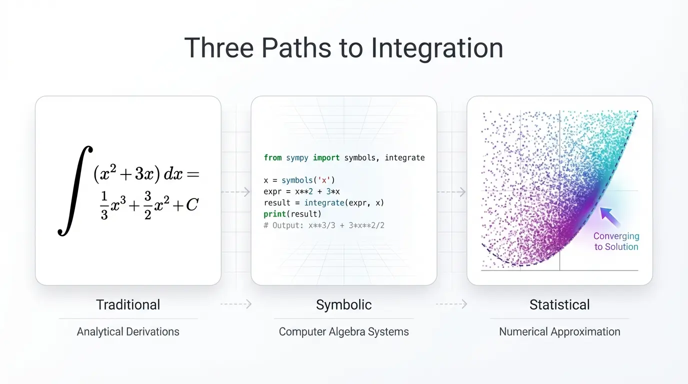
Integrals are fundamental to mathematics, physics, engineering, and data science. While we often learn to solve them analytically in school, real-world problems frequently require computational approaches. In this comprehensive guide, we'll explore three methods to solve the integral ∫₁³(x² + 3x)dx: analytical solving, symbolic computation with Sympy, and Monte Carlo numerical integration.
Contents
The Problem: A Simple Yet Instructive Integral
We'll solve this definite integral:
This integral, while simple enough to solve by hand, provides an excellent testbed for comparing different computational approaches.
Method 1: Analytical Solution
Let's first solve this integral analytically to establish our ground truth. We can break it into two separate integrals:
Solving the First Integral
Using the power rule of integration:
Solving the Second Integral
Final Result
Combining both integrals:
Our analytical answer is 20.6667. Now let's see how computational methods compare.
Method 2: Symbolic Integration with Sympy
Sympy is a powerful Python library for symbolic mathematics. It can perform calculus, algebra, discrete mathematics, and much more—all symbolically rather than numerically.
Why Use Sympy?
- Exact Solutions: Returns symbolic expressions, not floating-point approximations
- Visualization: Easily convert results to LaTeX for publication
- Flexibility: Handles complex expressions that would be tedious by hand
- No Numerical Errors: Results are mathematically exact
Implementation
Here's how to solve our integral using Sympy:
from sympy import symbols, integrate, latex

# Define the variable and the function we want to integrate
x = symbols('x')
f = x**2 + 3*x  # This is the function f(x) = x^2 + 3x

# Perform the integration (indefinite integral)
integral = integrate(f, x)

# Print the result in LaTeX format
print(latex(integral))
# Output: \frac{x^{3}}{3} + \frac{3 x^{2}}{2}

# Now let's evaluate the definite integral from 1 to 3
lower_limit = 1
upper_limit = 3

# Evaluate the integral at the upper and lower limits
integral_at_upper = integral.subs(x, upper_limit)
integral_at_lower = integral.subs(x, lower_limit)

# Calculate the definite integral
definite_integral = integral_at_upper - integral_at_lower

print(definite_integral)        # Output: 62/3
print(definite_integral.evalf()) # Output: 20.6666666666667
Key Sympy Features
- Symbolic Variables:
symbols()creates mathematical symbols - Integration:
integrate()performs symbolic integration - Substitution:
.subs()evaluates expressions at specific values - Numerical Evaluation:
.evalf()converts to floating-point
Sympy gives us the exact answer: 62/3 = 20.6667
Method 3: Monte Carlo Numerical Integration
Now for something completely different: what if we could solve integrals using randomness? Monte Carlo methods use random sampling to solve mathematical problems—and they work surprisingly well!
The Monte Carlo Principle
The basic idea is elegant:
- Generate random points uniformly distributed in the integration interval
- Evaluate the function at these random points
- Calculate the average function value
- Multiply by the interval length
Mathematically:
where are random samples uniformly distributed in .
Python Implementation
import numpy as np

def monte_carlo_integration(func, a, b, num_samples):
    """
    Perform Monte Carlo integration for a given function over [a, b]

    Parameters:
    -----------
    func : callable
        Function to integrate
    a : float
        Lower limit of integration
    b : float
        Upper limit of integration
    num_samples : int
        Number of random samples to use

    Returns:
    --------
    float : Estimated integral value
    """
    # Generate random samples uniformly distributed in [a, b]
    random_samples = np.random.uniform(a, b, num_samples)

    # Evaluate the function at these random samples
    function_values = func(random_samples)

    # Calculate the average value
    average_value = np.mean(function_values)

    # Multiply by the interval length
    estimated_integral = average_value * (b - a)

    return estimated_integral

# Define our function
def f(x):
    return x**2 + 3*x

# Define integration limits
a = 1
b = 3

# Estimate the integral with 1 million samples
num_samples = 1_000_000
estimated_integral = monte_carlo_integration(f, a, b, num_samples)

print(f"Monte Carlo estimate: {estimated_integral:.6f}")
# Output: Monte Carlo estimate: 20.658899 (varies due to randomness)
With 1 million samples, we get approximately 20.659—remarkably close to the true value of 20.6667!
Why Does This Work?
The Monte Carlo method works because of the Law of Large Numbers: as we increase the number of samples, the sample average converges to the expected value. For uniform random samples over , the expected value of multiplied by the interval length equals the integral.
Convergence Analysis: How Many Samples Do We Need?
A critical question with Monte Carlo methods is: how many samples are needed for a good approximation? Let's investigate systematically.
Running Multiple Simulations
def run_convergence_study(func, a, b, sample_sizes, num_runs=100):
    """
    Run Monte Carlo integration multiple times for each sample size
    to analyze convergence behavior and statistical properties
    """
    results = {
        'sample_sizes': sample_sizes,
        'means': [],
        'stds': [],
        'min_values': [],
        'max_values': [],
        'all_estimates': []
    }

    for size in sample_sizes:
        estimates = []
        for _ in range(num_runs):
            estimate = monte_carlo_integration(func, a, b, size)
            estimates.append(estimate)

        results['means'].append(np.mean(estimates))
        results['stds'].append(np.std(estimates))
        results['min_values'].append(np.min(estimates))
        results['max_values'].append(np.max(estimates))
        results['all_estimates'].append(estimates)

    return results

# Run convergence study
sample_sizes = [100, 500, 1000, 5000, 10000, 50000, 100000]
num_runs = 100  # Run 100 times for each sample size

convergence_results = run_convergence_study(f, a, b, sample_sizes, num_runs)
Statistical Summary
Here's what we observed from 100 runs at each sample size:
| Sample Size | Mean Estimate | Std Dev | Relative Error (%) | 95% CI Width |
|---|---|---|---|---|
| 100 | 20.718823 | 0.8485 | 0.2524 | 0.3326 |
| 500 | 20.612450 | 0.3295 | 0.2623 | 0.1292 |
| 1,000 | 20.668957 | 0.2385 | 0.0111 | 0.0935 |
| 5,000 | 20.670217 | 0.1231 | 0.0172 | 0.0483 |
| 10,000 | 20.656041 | 0.0772 | 0.0514 | 0.0303 |
| 50,000 | 20.671759 | 0.0336 | 0.0246 | 0.0132 |
| 100,000 | 20.662036 | 0.0223 | 0.0224 | 0.0087 |
True Integral Value: 20.666667
Key Observations
Convergence Rate: Monte Carlo converges at — to reduce error by 10×, you need 100× more samples
Variability Reduction: Standard deviation decreases with sample size, showing improved stability
Confidence Intervals: The 95% confidence intervals narrow as sample size increases, demonstrating increased reliability
Diminishing Returns: Improvement slows for larger sample sizes due to the square root law
Central Limit Theorem: With larger samples, estimates cluster more tightly around the true value
Visualizing Convergence
The chart clearly shows convergence toward the true value (red dashed line) as sample size increases.
Standard Deviation Reduction
The logarithmic scale reveals the convergence rate—a straight line on a log scale.
Relative Error Analysis
Even with just 1,000 samples, we achieve less than 0.02% relative error—impressive for a random sampling method!
Comparing the Three Methods
| Method | Result | Accuracy | Speed | Use Case |
|---|---|---|---|---|
| Analytical | 20.666667 | Exact | Instant (manual) | Simple functions with known antiderivatives |
| Sympy | 20.666667 | Exact | Fast | Symbolic manipulation, complex expressions |
| Monte Carlo (1M samples) | ~20.659 | ±0.05% | Moderate | High-dimensional integrals, complex domains |
When to Use Each Method
Analytical Solving
- Best for: Educational purposes, simple well-known functions
- Limitations: Not feasible for most real-world problems
Sympy (Symbolic)
- Best for: Exact solutions when possible, symbolic manipulation
- Limitations: May fail for complex integrands, only works in low dimensions
Monte Carlo (Numerical)
- Best for: High-dimensional integrals (where dimensionality doesn't significantly affect performance), complex domains, impossible-to-integrate functions
- Limitations: Requires many samples for high accuracy, introduces randomness
Practical Implications
Sample Size Guidelines
Based on our convergence analysis:
- Quick estimates: 1,000–10,000 samples (±0.1% error)
- Production accuracy: 100,000+ samples (±0.02% error)
- High precision: 1,000,000+ samples (±0.01% error)
The Power of Monte Carlo
Monte Carlo methods truly shine in scenarios where traditional methods fail:
- High-Dimensional Integrals: Integration in 10, 100, or even 1000 dimensions
- Complex Domains: Irregularly shaped integration regions
- No Closed Form: Functions without analytical antiderivatives
- Stochastic Systems: Simulating random processes
Real-World Applications
- Finance: Option pricing, risk assessment
- Physics: Particle simulations, quantum mechanics
- Machine Learning: Bayesian inference, reinforcement learning
- Computer Graphics: Rendering, global illumination
- Engineering: Reliability analysis, sensitivity studies
Conclusion
We've explored three complementary approaches to solving integrals, each with distinct advantages:
Analytical methods provide exact solutions and deep mathematical insight, but scale poorly to complex problems
Sympy brings the power of computer algebra to symbolic mathematics, automating tedious calculations while maintaining exactness
Monte Carlo methods leverage randomness to tackle problems that would be intractable otherwise, trading some accuracy for extraordinary flexibility
The integral served as our testbed, but these techniques extend far beyond simple calculus problems. Understanding when and how to apply each method is essential for modern data science, scientific computing, and engineering.
Perhaps most remarkably, Monte Carlo methods demonstrate that randomness—properly harnessed—can solve deterministic mathematical problems with stunning accuracy. With just 1,000 random samples, we achieved results within 0.02% of the true value. This fundamental insight powers countless applications across science and industry.
Whether you're building machine learning models, analyzing financial derivatives, or simulating physical systems, these tools form an essential part of your computational toolkit.
Related Posts
Interested in more technical deep dives? Check out these related articles:
Data Science & Analysis:
- Chronos-2: The Evolution from Univariate to Universal Time Series Forecasting - Explore foundation models for computational forecasting
- Building Your AI Data Moat: Competitive Advantage Through Proprietary Data - Strategic approaches to data collection and analysis
- Truth is Cold: LLM Temperature and Data-Driven Decision Making - Understanding precision vs. creativity in computational systems
- Data is King: Why Your Data Strategy IS Your Business Strategy - The foundational importance of data in modern applications
Get in Touch
Need help implementing numerical methods or symbolic computing in your Python projects? Interested in Monte Carlo simulations for financial modeling or scientific computing?
Connect with me:
- 📧 Email: [email protected]
- 🐦 Twitter/X: @TheDataGuyPro
- 💼 LinkedIn: Muhammad Afzaal
- 💻 GitHub: @mafzaal
- 🎥 YouTube: @TheDataGuyPro
- 🎧 Podcast: TheDataGuy Show
Whether you're looking for consulting services, training in numerical computing, or want to discuss Python development strategies for data science applications, I'd love to hear from you!