From Pollen Grains to Nuclear Bombs: The Astonishing Story of Monte Carlo Methods

It started with a botanist staring through a microscope, utterly baffled.

Edinburgh, 1827. Scottish botanist Robert Brown is observing pollen grains suspended in water — standard scientific work for the era. But what he sees makes no sense. The tiny particles are dancing. Zigzagging. Jerking unpredictably in every direction. No current, no wind, no force he can identify should make them move this way.

Brown does what any good scientist does: he rules out every possible explanation. Dead pollen — still moves. Volcanic ash — moves. Fragments of the Sphinx brought back from Egypt — still moves. Even powdered meteorites suspended in water show the same perpetual, restless jitter.

He can't explain it. He publishes his findings, notes his bafflement honestly, and moves on. The mystery would outlive him by 28 years.

What Brown witnessed that day in Edinburgh connects — through one of the most extraordinary chains of ideas in scientific history — to the hydrogen bomb, the Casino of Monaco, a sick mathematician's card game, and ultimately to the GPS in your smartphone, the algorithm behind Netflix's recommendations, and the risk models used every day on Wall Street.

This is the story of Monte Carlo methods: how randomness, properly harnessed, became one of humanity's most powerful tools for solving problems that were otherwise impossible.

This post continues our series on Monte Carlo methods. If you haven't already, check out From Symbolic Math to Random Sampling where we implement Monte Carlo integration hands-on in Python. Here, we tell the remarkable human story behind the technique.

Contents

---

The 80-Year Mystery No One Could Solve

Brown's mystery persisted through most of the nineteenth century. And it wasn't for lack of trying.

The phenomenon — later named Brownian motion in his honor — was meticulously documented, replicated, and studied across Europe. Generations of scientists offered explanations: temperature gradients, evaporation, electrical effects, capillary forces, even vital forces from exotic biological matter. Brown himself eliminated each of these, one by one, with the same careful rigor.

The deeper problem was philosophical. Classical physics — Newtonian mechanics, the pride of the Enlightenment — described the world as fundamentally deterministic. Given the position and velocity of every particle in a system, you could, in principle, calculate the entire future of that system. Randomness, in this worldview, was not a fundamental property of nature; it was just a measure of human ignorance.

But Brownian motion looked genuinely, irreducibly random. The particles didn't just move — they moved without memory, without pattern, without direction. Each jerk was independent of the last.

For determinism to survive, thermodynamics needed to explain this apparent randomness. And for thermodynamics to explain it, atoms — still a hotly debated hypothesis in the mid-1800s — had to actually exist.

It would take eighty years, a Danish astronomer studying stock markets, a young French mathematician obsessed with speculation, and eventually Albert Einstein's miraculous year to finally crack it open.

---

The Speculator Who Beat Einstein

In 1880, a Danish astronomer and mathematician named Thorvald Thiele published a paper on time series analysis. Hidden inside, almost incidentally, was what we'd recognize today as the first mathematical model of Brownian motion. But Thiele was thinking about something completely different — he was trying to capture the noise in astronomical measurements, the unexplained jitter in data that good scientists normally tried to remove.

He saw it as interference. A problem to be eliminated.

Twenty years later, a young French mathematician would look at essentially the same phenomenon and see it as the answer.

---

The Tragedy of Louis Bachelier

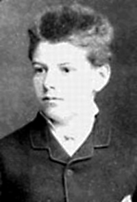
On March 29, 1900, at the Sorbonne in Paris, a student named Louis Bachelier defended his doctoral thesis: "Théorie de la Spéculation" — the Theory of Speculation.

The subject was not physics. It was not even mathematics in the traditional sense. Bachelier was studying the Paris stock market.

His core insight was both simple and revolutionary: the fluctuations in stock prices behave like a random walk. Small changes in price over a short interval are independent of the current price level. The market has no memory. Buyers and sellers are so evenly matched in their contradictory opinions that — mathematically — the expected return of any speculator is zero.

To model this, Bachelier reached for Gauss's probability distribution — the familiar bell curve — and applied it to the increments of stock prices. He developed what we'd now call the mathematics of stochastic processes and derived, from first principles, formulas for pricing financial options.

This was five years before Albert Einstein would publish his own analysis of random motion. Bachelier had effectively solved the mathematics of Brownian motion — from the Paris stock exchange.

His examiner, the legendary Henri Poincaré, was impressed by the originality but reserved in his praise. Poincaré saw the approach as clever but outside the mainstream. The thesis received a grade of "honorable" rather than the "very honorable" required for the best academic positions.

Bachelier's career never recovered. His academic path was interrupted by World War I. He spent decades in temporary positions, perpetually on the margins. He was finally awarded a permanent professorship in 1927, at age 57, at the University of Besançon — not exactly the pinnacle of French academia.

He remained obscure until the mid-1950s, when L.J. Savage, an American statistician, stumbled across his 1900 thesis and recognized it for what it was. Savage wrote to Paul Samuelson at MIT. Samuelson tracked down the work, was astonished, and began championing it.

By the 1960s and 70s, Bachelier's ideas had become the mathematical blood running through the veins of modern finance. Robert Merton, Fisher Black, Myron Scholes — all Nobel laureates — built directly on his foundation. Eugene Fama's efficient market hypothesis is, in many ways, a refinement of Bachelier's zero-expectation principle.

He never knew he had changed the world.

---

The Year Everything Changed

By 1905, the physics community was in open debate over whether atoms were real. Not a debate about sizes or shapes — a debate about existence. Serious scientists on both sides.

Then Albert Einstein published four papers in a single year that collectively dismantled the old order and built a new one. Most people remember two of them: the special theory of relativity and the explanation of the photoelectric effect (which won him the Nobel Prize).

Fewer people know about the third.

---

Einstein and the Dancing Particles

Einstein hadn't been particularly focused on Brownian motion. He was interested in thermodynamics, in the kinetic theory of matter, in what molecules would actually do if they existed — how their thermal energy would manifest at observable scales.

He reasoned from first principles: if molecules exist and are in constant thermal motion, they would continuously bombard any object suspended in fluid. Not smoothly, but in irregular, random bursts from all directions. The net force at any moment would be small, random, and memoryless.

This was exactly what Brown had seen.

Einstein connected the invisible (molecular collisions) to the visible (particle motion). He proved that the mean-square displacement of a particle — how far it wanders from its starting point on average — grows proportionally with time. Not with velocity. With time.

This was testable. This was quantitative. This was exactly the kind of prediction that could confirm or deny atomic theory.

Critically: Einstein's analysis also gave a way to calculate Avogadro's number — the number of atoms in a mole of substance — from measuring how far particles drift under a microscope. You could count atoms indirectly by watching pollen dance.

Within a few years, Jean Baptiste Perrin performed the optical measurements, confirmed Einstein's predictions exactly, and won the Nobel Prize for it. Atoms were real. The determinists lost.

---

Smoluchowski's Independent Confirmation

In 1906, Marian von Smoluchowski, a Polish physicist, published his own independent analysis. Smoluchowski knew the experimental data intimately — he had watched particles under microscopes far more than Einstein had — and he brought a different perspective.

Where Einstein worked from theory toward prediction, Smoluchowski worked backward from observation to mechanism. He calculated that a particle in a gas experiences approximately $10^{21}$ collisions per second. In liquid, even more. The sheer statistical weight of all those independent random kicks produced, in aggregate, the smooth-looking but fundamentally random drift that Brown had observed.

Smoluchowski made a point that proved philosophically important: depending on your perspective, the same phenomenon could appear three entirely different ways.

From far away, it looked like diffusion — a predictable, smooth spreading out of particles following precise differential equations.

Under a microscope, it looked like Brownian motion — the erratic, individual path of a single particle.

From a statistician's view, it was stochastic fluctuation — the collective behavior of countless independent random events.

---

Taming Infinity: The Mathematical Foundation

By 1905, physicists understood why particles jitter. But the mathematical description was still heuristic — a set of equations that worked without a rigorous foundation.

To make it rigorous, you needed to put a probability measure on something genuinely infinite: the space of all continuous paths a particle might trace. How do you assign probabilities to curves?

This wasn't a physics problem anymore. It was pure mathematics: the frontier where analysis, set theory, and probability intersect.

---

Enter Norbert Wiener

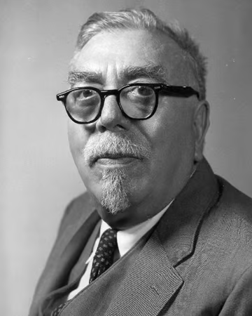
Norbert Wiener was, by most accounts, one of the most unusual mathematical minds of the twentieth century. A genuine child prodigy — reading by age 3, college graduate at 14 — he spent his career at MIT building bridges between pure mathematics and engineering.

In 1923, he published a paper titled "Differential Space" that solved the problem elegantly and completely.

Wiener proved that you can put a probability measure on the space of continuous functions — that is, you can talk meaningfully about the probability of a particle tracing any particular path. The resulting measure is now called the Wiener measure, and the process it describes — formally known as the Wiener process, informally as Brownian motion — has four defining properties:

1. It starts at zero
2. Future increments are independent of past values (no memory)
3. Steps over any time interval are normally distributed, with variance equal to elapsed time
4. The paths are continuous — the particle never teleports

The fourth property hides something subtle and beautiful: Wiener proved that although the paths are continuous — the particle is always somewhere — they are nowhere differentiable. You cannot draw a tangent line to a Brownian path at any point. It is infinitely jagged at every scale, like a coastline that gets more irregular the closer you zoom in.

This was mathematically astonishing. Physically, it made perfect sense: the particle's direction changes constantly, millions of times per second, with no smooth local behavior at any scale.

---

War Work and Cybernetics

Two decades later, Wiener's expertise in random processes took on urgent practical importance.

During World War II, both the Allies and Axis powers were grappling with the problem of anti-aircraft fire. Aircraft were fast. The angle of a gun had to lead the target — point where the plane would be by the time shells arrived, not where it was when you fired. At the ranges and speeds involved, this was a difficult prediction problem.

Wiener was recruited to solve it. He modeled an aircraft's path as a stochastic process: a series of measurements where each new position was correlated with — but not perfectly predicted by — the previous one. A pilot trying to evade made seemingly random corrections, and the gunner had to filter this noisy signal to predict future positions.

Wiener's solution introduced feedback loops: mechanisms where real-time data continuously adjusts the system's behavior. The gun didn't just predict once and fire — it constantly updated its prediction as new measurements came in.

This work, conducted under wartime secrecy, laid the foundations for what Wiener would later call cybernetics — the science of control and communication in animals and machines. His 1948 book, Cybernetics, would influence every field from engineering to neuroscience to economics.

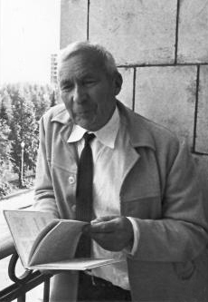
Meanwhile, in the Soviet Union, mathematician Andrey Kolmogorov was independently developing the rigorous analytic theory of stochastic processes — how probabilities evolve over time for Markov systems. The two streams — Wiener's path-based approach and Kolmogorov's equation-based approach — were equivalent, it turned out, just viewed from different angles.

The mathematical infrastructure for randomness was now complete. But the hardest problems were still insoluble.

---

The Solitaire Game That Changed Computing

Los Alamos, New Mexico. 1946.

The war is over, but the laboratory that built the atomic bomb is still very much in business. Physicists and mathematicians from across the world — many of them European refugees who had fled fascism — are working on the next problem: the hydrogen bomb, potentially a thousand times more powerful than the device dropped on Hiroshima.

To design it, you needed to solve a problem that was, by conventional mathematics, essentially impossible.

---

The Problem No Equation Could Solve

Consider a neutron moving through fissionable material. It travels some distance. It collides with an atomic nucleus. Depending on the collision, it might be absorbed, it might scatter at some angle, it might trigger fission and release more neutrons.

Each of those secondary neutrons does the same thing. And the tertiary neutrons. And so on, in a branching chain reaction where each step depends on random quantum events.

To calculate whether a given weapon design would achieve critical mass — whether the chain reaction would sustain and amplify — you needed to track the collective behavior of millions of neutrons, each following legitimately random paths through matter, all interacting with each other.

The equations describing this process were exponentially complex. You couldn't solve them on paper. You couldn't solve them with the mechanical calculators of the era, even if you had years to run them. The problem was, in a precise mathematical sense, intractable by deterministic methods.

The physicists were stuck.

---

A Sick Mathematician and a Card Game

Stanislaw Ulam was not feeling well.

The Polish mathematician — who had been at Los Alamos since the Manhattan Project — was recovering from encephalitis in early 1946, confined to bed with time to kill. He was dealing cards, playing Canfield solitaire, when a question drifted into his mind:

What are the odds that this particular hand will succeed?

He thought about it. The combinatorics of a single Canfield hand are extraordinarily complex — 52! possible orderings of the deck, with the rules creating dependencies between choices at each step. Computing the exact probability analytically would be enormously difficult.

But then: what if he just played the game 100 times, or 1,000 times, and counted? He wouldn't need to calculate the exact probability. He'd just estimate it from direct observation. For a quick answer — "roughly 1 in 3?" or "roughly 1 in 7?" — the counting approach would work far better.

The leap to physics was immediate.

If you could estimate the probability of a solitaire hand by randomly dealing many games and counting outcomes, you could estimate neutron diffusion paths by randomly sampling many possible trajectories and averaging the results.

You wouldn't solve the equations. You'd skip past them.

You wouldn't say, "Here is the exact behavior of every particle." You'd say, "Here is what happens on average when I sample the behavior randomly many times — and by the law of large numbers, that average will converge to the true answer."

Ulam recognized immediately that this was something new. The era of electronic computers was just beginning — the ENIAC had been completed the previous year. For the first time, a machine could generate and process thousands of random samples in reasonable time.

---

Von Neumann's Letter

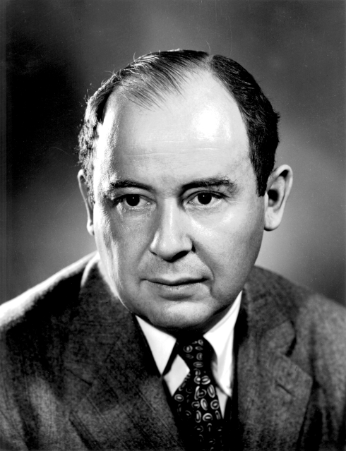
Ulam shared the idea with John von Neumann — arguably the most powerful mathematical mind of the twentieth century, and the person best positioned to act on it.

Von Neumann saw the potential immediately. He had been thinking about computing differently since a chance meeting at a train station in 1944, where he'd encountered an engineer working on the ENIAC. That meeting had set him on a path toward understanding what electronic computers might actually do, beyond their original purpose of computing artillery tables.

On March 11, 1947, von Neumann wrote a handwritten letter to Robert Richtmyer, the head of the Theoretical Division at Los Alamos. The letter contained the first formal written description of a Monte Carlo computation for an electronic computer — a detailed outline of how to use statistical sampling to solve the neutron diffusion problem.

This letter is one of the founding documents of computational science.

---

The Team, the Name, and the Machine

The work moved fast. Von Neumann mobilized resources. A team formed.

Nicholas Metropolis — a physicist and mathematician from Chicago who had joined Los Alamos during the war — was given responsibility for implementing the computational side. He named the method.

The research was classified. A code name was required. Metropolis knew that Ulam's uncle, a man of considerable appetite for gambling, had a habit of borrowing money from relatives so he could visit the Casino de Monte-Carlo in Monaco.

"Monte Carlo" captured everything about the method: games of chance, randomness quantified, probability made actionable. The name stuck.

Klára von Neumann — John's wife, a mathematician in her own right — did much of the actual programming for the early Monte Carlo calculations. She and Metropolis traveled to Maryland and worked for days without stopping on the ENIAC, manually modifying the machine's configuration to run the calculations.

By 1948, Metropolis had led the design and construction of the MANIAC — the Mathematical Analyzer Numerical Integrator and Automatic Computer — built specifically to run the kind of large-scale random sampling calculations that Monte Carlo required.

The H-bomb's feasibility calculations ran on it. Monte Carlo had proven itself on the hardest problem the era could produce.

---

Why It Works: The Law of Large Numbers

The mathematical justification for Monte Carlo is ancient, going back to Jacob Bernoulli in the 17th century: the Law of Large Numbers.

If you have a quantity you want to estimate — the probability of a solitaire hand succeeding, the average distance a neutron travels, the value of an integral — you can estimate it by sampling randomly and averaging. As the number of samples grows, your estimate converges to the true value. The error shrinks proportionally to $\frac{1}{\sqrt{n}}$:

$$\text{Error}\propto \frac{1}{\sqrt{n}}$$

This means 100 samples gets you to 10% error. To halve the error, you need four times as many samples — 400. To get to 1% error, 10,000 samples. It's slow convergence, but it's reliable convergence, and crucially, the convergence rate doesn't depend on the dimensionality of the problem.

This last point is everything. For deterministic numerical methods, error typically scales as $h^p$ where $h$ is the grid spacing and $p$ is the order of the method — but the number of grid points grows exponentially with the number of dimensions. A problem in 10 dimensions with 100 points per dimension requires $100^{10}=10^{20}$ points. Impossible.

---

From the Bomb to Everywhere

The Cold War demands that drove Monte Carlo's creation didn't hold it hostage. Within years of Ulam's breakthrough, the method had escaped the desert laboratory and begun spreading across science, engineering, and eventually industry.

---

The 1950s: First Wave of Expansion

Operations research — the discipline of making complex logistical decisions — adopted Monte Carlo almost immediately. If you needed to simulate a supply chain, a queueing system, a military logistics network, you could now model the inherent randomness rather than averaging it away.

In molecular chemistry, Marshall and Arianna Rosenbluth published their landmark 1955 paper pioneering Monte Carlo methods for simulating molecular systems. Their algorithm — still used today in modified form — enabled the first computer simulations of how molecules arrange themselves in space. This would eventually enable computational drug discovery, protein folding research, and materials science.

Alan Turing, in his 1950 paper on machine intelligence and in subsequent work through 1954, explored genetic algorithms and evolutionary computation — methods that use random mutation and selection to optimize complex systems. These are probabilistic search methods at heart, Monte Carlo in spirit.

---

The Mathematical Machinery: Stochastic Differential Equations

While Monte Carlo was conquering applications, mathematicians were building a deeper theoretical framework: stochastic differential equations (SDEs), a way of writing differential equations that include a random term.

Kiyosi Itô, a Japanese mathematician working in the 1940s, pioneered this field. He wanted to construct random processes that evolved continuously in time — think of a stock price drifting upward on average while jittering randomly around that trend.

The problem: you can't just add a random term to a normal differential equation. Brownian motion, as Wiener proved, is nowhere differentiable. The standard chain rule of calculus breaks down.

Itô developed new rules of calculus — now called Itô calculus — that correctly handle stochastic terms. The key result is Itô's lemma, a modified chain rule that includes an extra correction term whenever randomness is involved. This extra term looks small but isn't — it changes fundamental results in ways that have enormous practical consequences in finance.

The Black-Scholes option pricing formula, for instance, is derived using Itô's lemma. Without Itô calculus, modern derivatives markets could not function.

But solving SDEs analytically is usually impossible. To simulate them, you need numerical methods.

---

Euler-Maruyama and Milstein: Making SDEs Computable

In 1955, Gisiro Maruyama published the first numerical method for solving stochastic differential equations. He had come to probability theory through studying Wiener's work on Brownian motion, recognized the importance of Itô's framework, and extended the classical Euler method of ordinary differential equations to the stochastic case.

Given an Itô SDE of the form:

$$d{Y}_t=a(Y_t,t)dt+b(Y_t,t)d{W}_t$$

The Euler-Maruyama method steps forward in time as:

$$Y_{n+1}=Y_n+a(Y_n,t_n)\Delta t+b(Y_n,t_n)\Delta W_n$$

where $\Delta W_n\sim \mathcal{N}(0,\Delta t)$ — a random draw from a normal distribution with variance equal to the time step.

It converges at order $O(\sqrt{\Delta t})$ — half the rate of the ordinary Euler method — because the randomness introduces unavoidable discretization error that only shrinks as the square root of the step size.

In 1974, Grigori Milstein published an improvement. His method adds a correction term that accounts for how the diffusion coefficient $b$ changes with position:

$$Y_{n+1}=Y_n+a(Y_n,t_n)\Delta t+b(Y_n,t_n)\Delta W_n+\frac{1}{2}b(Y_n,t_n)b^{\prime }(Y_n,t_n)\left[(\Delta W_n{)}^2-\Delta t\right]$$

This extra term doubles the strong convergence order to $O(\Delta t)$ — much better for simulations that need to track individual paths accurately.

---

The 1990s: Particle Filters and Modern Bayesian Methods

By the 1990s, Monte Carlo had been productively colonizing new fields for four decades. But a new frontier emerged: real-time estimation of hidden states from noisy measurements — exactly the problem Wiener had worked on with anti-aircraft guns, but now with the computational power to do it properly.

In 1993, Gordon, Salmond, and Smith published the "bootstrap filter" — the first application of sequential Monte Carlo methods (now called particle filters) to Bayesian statistical inference. The idea: instead of tracking a single estimate of a hidden state, maintain thousands of random hypotheses ("particles"), each weighted by how well it matches observed data. Update the weights as new data arrives. Occasionally resample to keep the particles concentrated where probability is high.

This is the algorithm running inside GPS receivers, tracking satellites and estimating position from noisy range measurements.

It's the algorithm in radar systems that track aircraft.

It's used by epidemiologists modeling the spread of COVID-19, estimating transmission rates from noisy case count data in real time.

In 1996, Pierre Del Moral provided the rigorous mathematical foundation for these particle algorithms, proving convergence and establishing the theoretical guarantees that eventually made them trustworthy enough for critical applications.

---

Consolidation: Kloeden and Platen's Landmark Book

The field reached a kind of intellectual maturity in 1992 when Peter Kloeden and Eckhard Platen published Numerical Solution of Stochastic Differential Equations — a comprehensive treatment of the entire field that brought together:

• High-order Taylor expansion methods
• Runge-Kutta adaptations for stochastic systems
• Implicit methods for stiff problems
• Variance reduction techniques
• Weak approximation methods for computing expectations

The book organized decades of scattered research into a coherent discipline and became the standard reference for anyone implementing SDE simulations. It marks the transition from Monte Carlo as a collection of clever tricks to Monte Carlo as a rigorous mathematical science.

---

The Human Legacy of Random Thinking

Stepping back from the technical history, the story of Monte Carlo methods is a story about how scientific progress actually works — which looks nothing like the textbook version.

---

Ideas Travel Unexpectedly

Louis Bachelier applied physics to finance and solved a physics problem five years before it was formally posed in physics. Robert Brown observed a physical phenomenon while doing biology. Ulam found the key to nuclear physics while recovering from illness and playing cards. Norbert Wiener's wartime work on anti-aircraft guns founded a field — cybernetics — that shapes AI and robotics today.

This should be a comfort and a challenge for everyone working at the technical frontier today. Your expertise in accounting, or medicine, or music, might be exactly what's missing from some open problem in machine learning. The most important ideas often come from outside.

---

Randomness Is a Feature, Not a Bug

Every major figure in this story had to make peace with something that felt, at first, like a limitation: that perfect deterministic knowledge was impossible, and that uncertainty properly modeled was the best you could do.

Brown couldn't explain the jitter. Einstein turned the jitter into a tool to weigh atoms. Bachelier turned market noise into a pricing formula. Ulam turned the impossibility of exact neutron calculations into an argument for statistical sampling.

This is deeply counterintuitive. Scientists, engineers, and analysts are trained to reduce uncertainty, to control variables, to eliminate noise. Monte Carlo says: sometimes uncertainty is the solution.

---

Who Gets Credit

The history of Monte Carlo is also a story about who gets recognized and who doesn't.

Thorvald Thiele arguably modeled Brownian motion before Bachelier, but his work was in Danish and largely invisible to the broader scientific community.

Louis Bachelier solved the core problem in 1900 but spent his best years in obscurity.

Klára von Neumann wrote critical code and ran critical computations on ENIAC — work that has historically received far less recognition than her husband's theoretical contributions.

Arianna Rosenbluth co-invented the Metropolis-Hastings algorithm (published in 1953 under the names Metropolis, Rosenbluth, Rosenbluth, Teller, and Teller) — a foundational Monte Carlo method used in countless applications today.

The history of science is not always just. But knowing who actually built these tools is important — not to assign blame, but to understand what innovation actually looks like. It's collaborative, interdisciplinary, and it happens in unexpected places, often to people who won't be famous for it.

---

The Key Figures: A Complete Timeline

---

What Comes Next

Monte Carlo methods are not a solved, closed chapter in the history of mathematics. They are actively evolving, and some of the most important applications are being developed right now.

Here's where we're going together in this series:

---

🔢 Deep Dive: Implementing Stochastic Differential Equations

Our previous post covered Monte Carlo integration hands-on. The next technical deep dive will implement:

• Euler-Maruyama from scratch in Python — simulate geometric Brownian motion
• Milstein method — improve convergence for state-dependent diffusion
• Real application — price European and Asian options on historical stock data
• Convergence analysis — visualize how error shrinks with smaller time steps

---

💰 Application: Monte Carlo for Financial Risk

We'll explore how every major bank and hedge fund uses Monte Carlo for:

• Value at Risk (VaR) — estimating maximum likely loss
• Option pricing — beyond Black-Scholes for exotic derivatives
• Portfolio stress testing — what happens in your worst-case scenario?
• Credit risk — modeling default probabilities in loan portfolios

---

🤖 Frontier: Monte Carlo in Machine Learning

Perhaps the most exciting current frontier — Monte Carlo methods are powering modern AI:

• Dropout as Monte Carlo sampling — uncertainty estimation in neural networks
• Variational inference — approximate Bayesian learning at scale
• Monte Carlo Tree Search — the algorithm that beat world champions at Go (AlphaGo)
• Reinforcement learning — how agents learn from random exploration

---

🧬 Applications: Medicine, Climate, and Engineering

Monte Carlo isn't just for physicists and quants. We'll cover:

• Radiation treatment planning — optimizing cancer therapy dose delivery
• Epidemic modeling — how epidemiologists estimated COVID-19 transmission in real time
• Climate ensemble predictions — why weather forecasts give probabilities, not certainties
• Boeing 787 structural analysis — how aerospace engineers certify wing designs without breaking planes

---

🧪 Historical Deep Dive: Bachelier's Revenge

The full story of Louis Bachelier deserves its own post — a biography of one of the most underappreciated figures in mathematical history. His arc from obscure thesis to the foundation of a multi-trillion-dollar derivatives market is one of science's great redemption stories.

---

Get in Touch

Writing and thinking seriously about Monte Carlo methods — their history, their mathematics, their modern applications — is one of the most intellectually satisfying things I do. If this post sparked something for you, I'd love to continue the conversation.

Whether you're a data scientist who now understands where the tools on your workbench actually came from, a finance professional wondering how to apply stochastic simulation to your own risk models, or simply someone who finds the sheer human drama of this history as compelling as I do — reach out.

Connect with me:

• 📧 Email: [email protected]
• 🐦 Twitter/X: @TheDataGuyPro
• 💼 LinkedIn: Muhammad Afzaal
• 💻 GitHub: @mafzaal
• 🎥 YouTube: @TheDataGuyPro
• 🎧 Podcast: TheDataGuy Show

Need help applying Monte Carlo methods to your organization's specific problems — risk modeling, scientific simulation, AI uncertainty quantification, or financial derivatives? That's consulting work I genuinely enjoy. Let's talk about what you're trying to solve.

---

Related Posts

The Monte Carlo Series:

• From Symbolic Math to Random Sampling: Mastering Integral Calculations with Python — Hands-on implementation of Monte Carlo integration

Data Science Foundations:

• Chronos-2: The Evolution from Univariate to Universal Time Series Forecasting — Probabilistic forecasting at scale
• Truth is Cold: LLM Temperature and Data-Driven Decision Making — Randomness and creativity in AI systems
• Building Your AI Data Moat: Competitive Advantage Through Proprietary Data — Strategic data thinking

History of Science:

• Data is King: Why Your Data Strategy IS Your Business Strategy — From Bachelier's markets to modern data strategy

---

References

1. 100 years of Einstein's Theory of Brownian Motion: from Pollen Grains to Protein Trains 1. Indian Academy of Sciences.
2. The theory of Brownian Motion: A Hundred Years' Anniversary. Institut für Physik, University of Augsburg.
3. Centenary of Marian Smoluchowski's Theory of Brownian Motion. University of Connecticut.
4. A short history of stochastic integration and mathematical finance: The early years, 1880--1970. Imperial College London.
5. Louis Bachelier's Theory of Speculation. Imperial College London.
6. Euler–Maruyama method. Wikipedia.
7. A Brief History of Runge-Kutta Methods. Clueless Fundatma.
8. Louis Bachelier's Theory Of Speculation: The Origins Of Modern Finance. Z/Yen.
9. Probability theory - part 4 brownian motion. IISc Math.
10. Norbert Wiener | Department of Mathematics. Tufts University.
11. Hitting the Jackpot: The Birth of the Monte Carlo Method. Los Alamos National Laboratory.
12. Monte Carlo method. Wikipedia.
13. Stochastic differential equation. Wikipedia.
14. Numerical Solution of Stochastic Differential Equations. Kloeden & Platen (1992), Google Books.
15. Milstein method. Wikipedia.